PRML 第2章 確率分布 ノンパラメトリック手法

パターン認識と機械学習、第2章からは「2.5.2 ノンパラメトリック手法」を実装します。

取り出してきたデータの数を数え上げて、確率分布を把握する手法が紹介されてます。
この章はあんまり時間かけてもしょうが無いなと感じたので、さくっと実装。
カーネル密度法もスクラッチせず、scipyのパッケージ使ってズルしました。

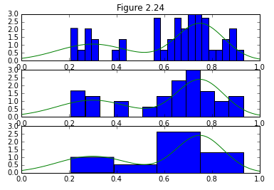
ヒストグラム・コード

import numpy as np
import matplotlib.pyplot as plt
from pylab import *
from scipy import stats
from scipy.stats.kde import gaussian_kde
import random

def mix_G(x):
    return (0.4 * G1 + 0.6 * G2)

def mix_G_distribution(n):
  ratio = 0.3
  if random.random() <ratio:
    return random.gauss(M1, S1)
  else:
    return random.gauss(M2, S2)

if __name__ == "__main__":
    x = np.linspace(0, 1, 100)

    # Set normal distribution1 
    M1 = 0.3
    S1 = 0.15
    G1 = stats.norm.pdf(x, M1, S1)

    # Set normal distribution1 
    M2 = 0.75
    S2 = 0.1
    G2 = stats.norm.pdf(x, M2, S2)

    N = 50
    Data = [mix_G_distribution(n) for n in range(N)]


    plt.subplot(3, 1, 1)
    plt.hist(Data, bins=1/0.04, normed=True)
    plt.plot(x, mix_G(x), "g-")
    plt.xlim(0, 1)
    plt.ylim(0, 3)
    title("Figure 2.24")

    plt.subplot(3, 1, 2)
    plt.hist(Data, bins=1/0.08, normed=True)
    plt.plot(x, mix_G(x), "g-")
    plt.xlim(0, 1)
    plt.ylim(0, 3)

    plt.subplot(3, 1, 3)
    plt.hist(Data, bins=1/0.25, normed=True)
    plt.plot(x, mix_G(x), "g-")
    plt.xlim(0, 1)
    plt.ylim(0, 3)

結果

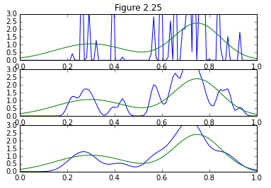
カーネル密度法・コード

if __name__ == "__main__":
    #Karnel density estimation
    from scipy.stats.kde import gaussian_kde

    plt.subplot(3, 1, 1)
    plt.plot(x, gaussian_kde(Data, 0.005)(x))
    plt.plot(x, mix_G(x), "g-")
    plt.xlim(0, 1)
    plt.ylim(0, 3)
    title("Figure 2.25")

    plt.subplot(3, 1, 2)
    plt.plot(x, gaussian_kde(Data, 0.07)(x))
    plt.plot(x, mix_G(x), "g-")
    plt.xlim(0, 1)
    plt.ylim(0, 3)

    plt.subplot(3, 1, 3)
    plt.plot(x, gaussian_kde(Data, 0.2)(x))
    plt.plot(x, mix_G(x), "g-")
    plt.xlim(0, 1)
    plt.ylim(0, 3)

結果

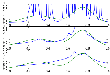
K近傍法・コード

#k_Neighbourhood
def k_NN(test, train, k):
    train = np.array(train)
    train.sort()
    r = []
    for i in test:
        distance = abs(train - i)
        distance.sort()
        r.append(distance[(k-1)])
    r = np.array(r)
    return k / (2* r * N)



if __name__ == "__main__":
    title("Figure 2.26")
    plt.subplot(3, 1, 1)
    plt.plot(x, k_NN(x, Data, 1))
    plt.plot(x, mix_G(x), "g-")
    plt.xlim(0, 1)
    plt.ylim(0, 3)

    plt.subplot(3, 1, 2)
    plt.plot(x, k_NN(x, Data, 10))
    plt.plot(x, mix_G(x), "g-")
    plt.xlim(0, 1)
    plt.ylim(0, 3)

    plt.subplot(3, 1, 3)
    plt.plot(x, k_NN(x, Data, 30))
    plt.plot(x, mix_G(x), "g-")
    plt.xlim(0, 1)
    plt.ylim(0, 3)

結果