PRML5章から図5.3を再現するために、ニューラルネットワークを実装してみます。
先に申し上げておきますと、偉そうに実装とか言ってるものの、コードから再現した図は歯切れの悪いものとなっております。。。不完全なものを上げるなと怒られそうな気もしますが、ご参考に下さい。
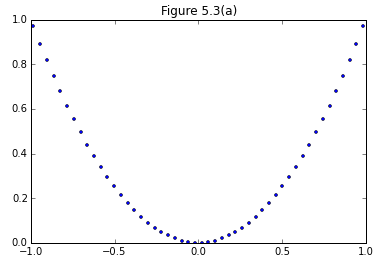
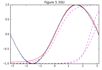
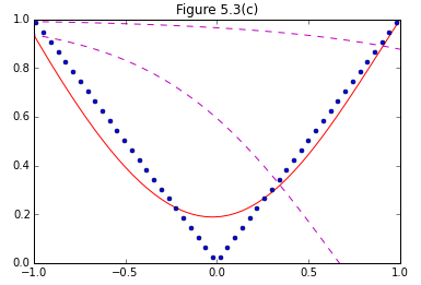
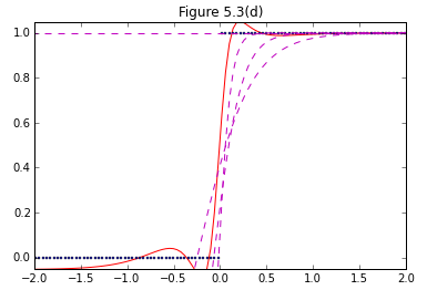
まず、図5.3(b),(c),(d)に関してはPRMLの中の図に比べて予測精度がいまいち良くない印象。さらに、図5.3(a)に関しては全く見当はずれな予測が返ってくるという状況。試行錯誤しましたが、力不足でして、どなたか間違い気づかれましたらご指摘下さい。
ニューラルネットワークや、誤差伝播法(Backpropagation)そのものの解説はPRMLやはじパタなどに任せるとして、実装に必要な部分だけざっと確認したいと思います。
実装の大まかな流れ
①ニューラルネットを経たアウトプットは(5.9)で表される。PRML文中の式は活性化関数$h()$にシグモイド関数を想定しているが、図5.3ではtanh()が指定されている点に注意。
y_k({\bf x}, {\bf w}) = \sigma(\sum_{j=0}^M, w^{(2)}_{kj} h(\sum_{i=0}^D w^{(1)}_{ji} x_i)) (5.9)
②ノード間の重み${\bf w}$を学習するにあたり、各ノードでのアウトプットと実測値との差を求める。まずは隠れユニットの出力は(5.63)、出力ユニットの出力は(5.64)。
z_j = {\rm tanh} (\sigma(\sum_{i=0}^D, w^{(1)}_{ji} x_i)) (5.63)
y_k = \sum_{j=0}^M, w^{(2)}_{kj} z_i (5.64)
③次に出力層での誤差$\delta_k$を求める。
\delta_k = y_k - t_k (5.65)
④次に隠れ層での誤差$\delta_j$を求める。
\delta_j = (1-{z_j}^2) \sum_{k=1}^K w_{kj} \delta_k (5.65)
⑤(5.43)、(5.67)を用いてノード間の重みを更新する。
{\bf w}^{\rm \tau+1} = {\bf w}^{\rm \tau} - \mu \nabla E({\bf{w}})(5.43)
コード
import matplotlib.pyplot as plt
from pylab import *
import numpy as np
import random

def heaviside(x):
    return 0.5 * (np.sign(x) + 1)

def NN(x_train, t, n_imput, n_hidden, n_output, eta, W1, W2, n_loop):
    for n in xrange(n_loop):
        for n in range(len(x_train)):
            x = np.array([x_train[n]])

            #feedforward
            X = np.insert(x, 0, 1) #Insert fixed term

            A = np.dot(W1, X) #(5.62)
            Z = np.tanh(A)  #(5.63)
            Z[0] = 1.0
            Y = np.dot(W2, Z) #(5.64)


            #Backprobagation
            D2 = Y - t[n]#(5.65)
            D1 = (1-Z**2)*W2*D2 #(5.66)

            W1 = W1- eta*D1.T*X #(5.67), (5.43)
            W2 = W2- eta*D2.T*Z #(5.67), (5.43)
    return  W1, W2

def output(x, W1, W2):
    X = np.insert(x, 0, 1) #Insert fixed term

    A = np.dot(W1, X) #(5.62)
    Z = np.tanh(A)  #(5.63)
    Z[0] = 1.0 #Insert fixed term
    Y = np.dot(W2, Z) #(5.64)
    return Y, Z

if __name__ == "__main__":
    #Set form of nueral network
    n_imput = 2
    n_hidden = 4
    n_output = 1
    eta = 0.1
    W1 = np.random.random((n_hidden, n_imput))
    W2 = np.random.random((n_output, n_hidden))
    n_loop = 1000


    #Set train data
    x_train = np.linspace(-4, 4, 300).reshape(300, 1)
    y_train_1 = x_train * x_train
    y_train_2 = np.sin(x_train)
    y_train_3 = np.abs(x_train)
    y_train_4 = heaviside(x_train)

    W1_1, W2_1= NN(x_train, y_train_1, n_imput, n_hidden, n_output, eta, W1, W2, n_loop)
    W1_2, W2_2= NN(x_train, y_train_2, n_imput, n_hidden, n_output, eta, W1, W2, n_loop)
    W1_3, W2_3= NN(x_train, y_train_3, n_imput, n_hidden, n_output, eta, W1, W2, n_loop)
    W1_4, W2_4= NN(x_train, y_train_4, n_imput, n_hidden, n_output, eta, W1, W2, n_loop)

    Y_1 = np.zeros((len(x_train), n_output))
    Z_1 = np.zeros((len(x_train), n_hidden))

    Y_2 = np.zeros((len(x_train), n_output))
    Z_2 = np.zeros((len(x_train), n_hidden))

    Y_3 = np.zeros((len(x_train), n_output))
    Z_3 = np.zeros((len(x_train), n_hidden))

    Y_4 = np.zeros((len(x_train), n_output))
    Z_4 = np.zeros((len(x_train), n_hidden))

    for n in range(len(x_train)):
        Y_1[n], Z_1[n] =output(x_train[n], W1_1, W2_1)
        Y_2[n], Z_2[n] =output(x_train[n], W1_2, W2_2)
        Y_3[n], Z_3[n] =output(x_train[n], W1_3, W2_3)
        Y_4[n], Z_4[n] =output(x_train[n], W1_4, W2_4)


    plt.plot(x_train, Y_1, "r-")
    plt.plot(x_train, y_train_1, "bo", markersize=3)
    for i in range(n_hidden):
        plt.plot(x_train, Z_1[:,i], 'm--')
    xlim([-1,1])
    ylim([0, 1])
    title("Figure 5.3(a)")
    show()

    plt.plot(x_train, Y_2, "r-")
    plt.plot(x_train, y_train_2, "bo", markersize=2)
    for i in range(n_hidden):
        plt.plot(x_train, Z_2[:,i], 'm--')
    xlim([-3.14,3.14])
    ylim([-1, 1])
    title("Figure 5.3(b)")
    show()


    plt.plot(x_train, Y_3, "r-")
    plt.plot(x_train, y_train_3, "bo", markersize=4)
    for i in range(n_hidden):
        plt.plot(x_train, Z_3[:,i], 'm--')
    xlim([-1,1])
    ylim([0, 1])
    title("Figure 5.3(c)")
    show()


    plt.plot(x_train, Y_4, "r-")
    plt.plot(x_train, y_train_4, "bo" ,markersize=2)
    for i in range(n_hidden):
        plt.plot(x_train, Z_4[:,i], 'm--')
    xlim([-2,2])
    ylim([-0.05, 1.05])
    title("Figure 5.3(d)")
    show()
結果