1年以上も前ですが、edXのScalable Machine learningを受講していた時のコードが出てきたので、見直してみました。この講座のネタが、KaggleのCriteoのコンペのデータ
を基にしたCTR予測でして、One-hot-encodingやhushingした高次元のデータを
Mllibのロジスティック回帰モデルで予測をするといったものです。今回は予測精度そのものよりも、ハッシュ関数で次元圧縮したものが、OHE化したデータと比べてどの程度予測精度に差が出るのかを見ていきます。
Sparkもかなり前のバージョンだったので、今ならまた違う実装の仕方があるような気もしますが、出来合いの機能に頼らずに実装したことで理解が深まった記憶があるので、そのまんま。追加機能の勉強兼ねた比較はまた別のタイミングで行いたいなと思います。 SparkはVirtualbox上にたてたUbuntuにインストールしたものをシングルノードで使用しています。
おおまかな手順
①データの準備
元データを訓練、評価、テストデータにそれぞれ分割
②元データにOHEを適用。ここで特徴量は20万以上になります。
③OHE後のデータでロジスティック回帰で分析(model1)
④ハッシュトリックで次元量の削減(およそ3,000程度)
⑤ハッシュ後のデータでロジスティック回帰分析
-Mllibデフォルト設定のモデル(model2)
-グリッドサーチでパラメータ設定したモデル(model3)
⑥Loglosによるモデル評価
-OHEデータモデル(model1) vs Hushingデータモデル(model2)
-Hushingデータ・デフォルトモデル(model2) vs Hushingデータ・GSモデル(model3)
コード
まずはデータを読み込んで分割、眺めてみます。
import numpy as np
from pyspark.mllib.linalg import SparseVector
from pyspark.mllib.regression import LabeledPoint

rawData = (sc.textFile("dac_sample.txt").map(lambda x: x.replace('\t', ',')))

OneSample = rawData.take(1)
print OneSample


weights = [.8, .1, .1]
seed = 42
rawTrainData, rawValidationData, rawTestData = rawData.randomSplit(weights, seed)

# Cache each datasets as it is used repeatedly
rawTrainData.cache()
rawValidationData.cache()
rawTestData.cache()

nTrain = rawTrainData.count()
nVal = rawValidationData.count()
nTest = rawTestData.count()
print nTrain, nVal, nTest, nTrain + nVal + nTest


[u'0,1,1,5,0,1382,4,15,2,181,1,2,,2,68fd1e64,80e26c9b,fb936136,7b4723c4,25c83c98,7e0ccccf,de7995b8,1f89b562,a73ee510,a8cd5504,b2cb9c98,37c9c164,2824a5f6,1adce6ef,8ba8b39a,891b62e7,e5ba7672,f54016b9,21ddcdc9,b1252a9d,07b5194c,,3a171ecb,c5c50484,e8b83407,9727dd16']
79911 10075 10014 100000
OHEを分割したデータに当てます。
def createOneHotDict(inputData):
    OHEDict = (inputData
               .flatMap(lambda x: x)
               .distinct()
               .zipWithIndex()
               .collectAsMap())
    return OHEDict


def parsePoint(point):
    items = point.split(',')
    return [(i, item) for i, item in enumerate(items[1:])]

def oneHotEncoding(rawFeats, OHEDict, numOHEFeats):
    sizeList = [OHEDict[f] for f in rawFeats if f in OHEDict]
    sortedSizeList = sorted(sizeList)
    valueList = [1 for f in rawFeats if f in OHEDict ]
    return SparseVector(numOHEFeats, sortedSizeList, valueList)


def parseOHEPoint(point, OHEDict, numOHEFeats):
    parsedPoints = parsePoint(point)
    items = point.split(',')
    label = items[0]
    features = oneHotEncoding(parsedPoints, OHEDict, numOHEFeats)
    return LabeledPoint(label, features)

parsedFeat = rawTrainData.map(parsePoint)
ctrOHEDict = createOneHotDict(parsedFeat)
numCtrOHEFeats = len(ctrOHEDict.keys())


OHETrainData = rawTrainData.map(lambda point: parseOHEPoint(point, ctrOHEDict, numCtrOHEFeats)).cache()
OHEValidationData = rawValidationData.map(lambda point: parseOHEPoint(point, ctrOHEDict, numCtrOHEFeats)).cache()
OHETestData = rawTestData.map(lambda point: parseOHEPoint(point, ctrOHEDict, numCtrOHEFeats)).cache()

print ('Feature size after OHE:\n\tNumber of features = {0}'
       .format(numCtrOHEFeats))

print OHETrainData.take(1)

Feature size after OHE:
	Number of features = 233286
[LabeledPoint(0.0, (233286,[386,3077,6799,8264,8862,11800,12802,16125,17551,18566,29331,33132,39525,55794,61786,81396,82659,93573,96929,100677,109699,110646,112132,120260,128596,132397,132803,140620,160675,185498,190370,191146,195925,202664,204273,206055,222737,225958,229942],[1.0,1.0,1.0,1.0,1.0,1.0,1.0,1.0,1.0,1.0,1.0,1.0,1.0,1.0,1.0,1.0,1.0,1.0,1.0,1.0,1.0,1.0,1.0,1.0,1.0,1.0,1.0,1.0,1.0,1.0,1.0,1.0,1.0,1.0,1.0,1.0,1.0,1.0,1.0]))]
OHE後のデータにてロジスティック回帰を実施。とりあえずパラメーター設定はデフォルトのままやってみます。
from pyspark.mllib.classification import LogisticRegressionWithSGD

numIters = 100
stepSize = 1.0
regParam = 0.01
regType = 'l2'
includeIntercept = True

model0 = LogisticRegressionWithSGD.train(data = OHETrainData,
                                         iterations = numIters,
                                         step = stepSize,
                                         regParam = regParam,
                                         regType = regType,
                                         intercept = includeIntercept)

# Compute loglos
from math import log, exp

def computeLogLoss(p, y):
    epsilon = 10e-12
    if y == 1:
        return -log(epsilon + p) if p == 0 else -log(p)
    elif y == 0:
        return -log(1 - p + epsilon) if p == 1 else -log(1 - p)

def getP(x, w, intercept):
    rawPrediction = x.dot(w) + intercept

    # Bound the raw prediction value
    rawPrediction = min(rawPrediction, 20)
    rawPrediction = max(rawPrediction, -20)
    return 1.0 / (1.0 + exp(-rawPrediction))

def evaluateResults(model, data):
    return data.map(lambda x: computeLogLoss(getP(x.features, model.weights, model.intercept), x.label)).sum() / data.count()

logLossValLR0 = evaluateResults(model0, OHEValidationData)
print ('Validation Logloss for model1:\n\t = {0}'
       .format(logLossValLR0))
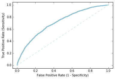
素うどんのロジスティック回帰でどこまで予測できてるか、ROC曲線を描いてみます。ぼちぼちの精度でできてるようでした。
labelsAndScores = OHEValidationData.map(lambda lp: (lp.label, getP(lp.features, model0.weights, model0.intercept)))
labelsAndWeights = labelsAndScores.collect()
labelsAndWeights.sort(key=lambda (k, v): v, reverse=True)
labelsByWeight = np.array([k for (k, v) in labelsAndWeights])

length = labelsByWeight.size
truePositives = labelsByWeight.cumsum()
numPositive = truePositives[-1]
falsePositives = np.arange(1.0, length + 1, 1.) - truePositives

truePositiveRate = truePositives / numPositive
falsePositiveRate = falsePositives / (length - numPositive)

import matplotlib.pyplot as plt
%matplotlib inline

fig = plt.figure()
ax = plt.subplot(111)

ax.set_xlim(-.05, 1.05), ax.set_ylim(-.05, 1.05)
ax.set_ylabel('True Positive Rate (Sensitivity)')
ax.set_xlabel('False Positive Rate (1 - Specificity)')
plt.plot(falsePositiveRate, truePositiveRate, color='#8cbfd0', linestyle='-', linewidth=3.)
plt.plot((0., 1.), (0., 1.), linestyle='--', color='#d6ebf2', linewidth=2.)
次に元データに対してハッシュトリックを当てます。
OHE後の次元数は20万程度、今回ハッシュ関数のバケット数を2の15乗で32768個としてます。
from collections import defaultdict
import hashlib

def hashFunction(numBuckets, rawFeats, printMapping=False):
    mapping = {}
    for ind, category in rawFeats:
        featureString = category + str(ind)
        mapping[featureString] = int(int(hashlib.md5(featureString).hexdigest(), 16) % numBuckets)
    sparseFeatures = defaultdict(float)
    for bucket in mapping.values():
        sparseFeatures[bucket] += 1.0
    return dict(sparseFeatures)


def parseHashPoint(point, numBuckets):
    parsedPoints = parsePoint(point)
    items = point.split(',')
    label = items[0]
    features = hashFunction(numBuckets, parsedPoints, printMapping=False)
    return LabeledPoint(label, SparseVector(numBuckets, features))

numBucketsCTR = 2 ** 15
hashTrainData = rawTrainData.map(lambda x: parseHashPoint(x, numBucketsCTR))
hashTrainData.cache()
hashValidationData = rawValidationData.map(lambda x: parseHashPoint(x, numBucketsCTR))
hashValidationData.cache()
hashTestData = rawTestData.map(lambda x: parseHashPoint(x, numBucketsCTR))
hashTestData.cache()

print ('Feature size after hushing:\n\tNumber of features = {0}'
       .format(numBucketsCTR))

print hashTrainData.take(1)

Feature size after hushing:
	Number of features = 32768
[LabeledPoint(0.0, (32768,[1305,2883,3807,4814,4866,4913,6952,7117,9985,10316,11512,11722,12365,13893,14735,15816,16198,17761,19274,21604,22256,22563,22785,24855,25202,25533,25721,26487,26656,27668,28211,29152,29402,29873,30039,31484,32493,32708],[1.0,1.0,1.0,1.0,1.0,1.0,1.0,1.0,1.0,1.0,1.0,1.0,1.0,1.0,1.0,1.0,1.0,1.0,1.0,1.0,1.0,1.0,1.0,1.0,1.0,1.0,1.0,1.0,1.0,1.0,1.0,1.0,1.0,1.0,1.0,1.0,1.0,1.0]))]
ハッシュ関数をあてた後のデータにてロジスティック分析。
デフォルト設定のものと、グリッドサーチでパラメータを探したものと二つモデルを作ります。
まずは素うどんの方から。
numIters = 100
stepSize = 1.0
regParam = 0.01
regType = 'l2'
includeIntercept = True

model1 = LogisticRegressionWithSGD.train(data = hashTrainData,
                                         iterations = numIters,
                                         step = stepSize,
                                         regParam = regParam,
                                         regType = regType,
                                         intercept = includeIntercept)

logLossValLR1 = evaluateResults(model1, hashValidationData)
print ('Validation Logloss for model1:\n\t = {0}'
       .format(logLossValLR1))

Validation Logloss for model1:
	 = 0.482691122185
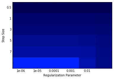
次にグリッドサーチを実施してパラメータを決めた後にモデル構築します。
numIters = 500
stepSizes = [0.1, 0.5, 1, 3, 5, 7]
regParams = [1e-7, 1e-6, 1e-5, 1e-4, 1e-3, 1e-2]
regType = 'l2'
includeIntercept = True


# Initialize variables using values from initial model training
bestModel = None
bestLogLoss = 1e10
logLoss = np.zeros((len(stepSizes),len(regParams)))

for i in xrange(len(stepSizes)):
    for j in xrange(len(regParams)):
        model = LogisticRegressionWithSGD.train(data = hashTrainData,
                                                iterations = numIters,
                                                step = stepSizes[i],
                                                regParam = regParams[j],
                                                regType = regType,
                                                intercept = includeIntercept)

        logLoss[i, j] = evaluateResults(model, hashValidationData)

        if (logLoss[i, j] < bestLogLoss):
            bestModel = model
            bestStepsize = stepSizes[i]
            bestParams = regParams[j]
            bestLogLoss = logLoss[i,j]


print ('best parameters:\n\tBest Stepsize = {0:.3f}\n\tBest Rarams = {1:.3f}'
       .format(bestStepsize, bestParams))

print bestParams,logLoss

%matplotlib inline
from matplotlib.colors import LinearSegmentedColormap


numRows, numCols = len(stepSizes), len(regParams)
logLoss = np.array(logLoss)
logLoss.shape = (numRows, numCols)

fig = plt.figure()
ax = plt.subplot(111)


ax.set_xticklabels(regParams), ax.set_yticklabels(stepSizes)
ax.set_xlabel('Regularization Parameter'), ax.set_ylabel('Step Size')

colors = LinearSegmentedColormap.from_list('blue', ['#0022ff', '#000055'], gamma=.2)
image = plt.imshow(logLoss,interpolation='nearest', aspect='auto',
                    cmap = colors)
pass

best parameters:
	Best Stepsize = 7.000
	Best Rarams = 0.000
1e-07 [[ 0.51910013  0.51910015  0.51910029  0.51910175  0.51911634  0.51926454]
 [ 0.48589729  0.4858974   0.48589847  0.48590921  0.48605802  0.48715278]
 [ 0.47476165  0.47476184  0.47476375  0.47478289  0.4750353   0.47731296]
 [ 0.46130496  0.46130542  0.46131004  0.46137622  0.46208485  0.46799094]
 [ 0.45587263  0.45587339  0.45588094  0.45600577  0.45715016  0.465792  ]
 [ 0.45268179  0.45268281  0.45270706  0.45286577  0.45438559  0.46488834]]
最期に下記の軸によるLoglosによるモデル評価です。
-OHEデータモデル(model1) vs Hushingデータモデル(model2)
-Hushingデータ・デフォルトモデル(model2) vs Hushingデータ・GSモデル(model3)
Loglossでの比較では、次元量を圧縮したHushing後のデータを使っても予測精度が落ちていませんね、面白いです。
logLossTestLR0 = evaluateResults(model0, OHETestData)
logLossTestLR1 = evaluateResults(model1, hashTestData)
logLossTestLRbest = evaluateResults(bestModel, hashTestData)

print ('OHECoding & Hashed Features Test Logloss:\n\tOHEModel = {0:.3f}\n\thashModel = {1:.3f}'
       .format(logLossTestLR0, logLossTestLR1))

print ('Hashed Features Validation Test Logloss:\n\tBaseModel = {0:.3f}\n\tBestModel = {1:.3f}'
       .format(logLossTestLR1, logLossTestLRbest))

OHECoding & Hashed Features Test Logloss:
	OHEModel = 0.490
	hashModel = 0.490
Hashed Features Validation Test Logloss:
	BaseModel = 0.490
	BestModel = 0.460