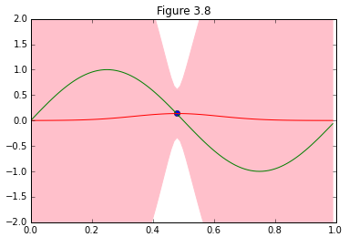
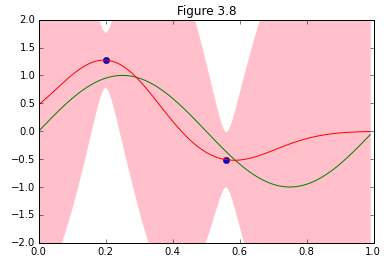
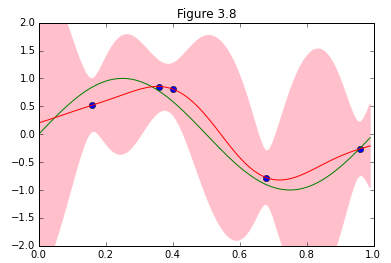
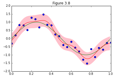
パターン認識と機械学習、第3章からベイズ線形回帰が予測分布を収束させていく様子を再現します。
やっていることは、1章でやったベイズ推定とほぼ一緒で、基底関数がガウス関数(3.4)になっているだけです。
ですので、コードもほぼほぼ流用してます。
1章と比較すると、3章では数式の表現がベクトルを扱うように書きなおされてますが、この辺何か意図あるのでしょうか。
(3.16)の特徴ベクトルの概念をここで紹介したからこの書き方なのかと思ってますが、どうなんでしょう。
実装の大まかな流れ
①求めたいのは予測分布(3.57)。
p(t|{\bf x}, {\bf t}, \alpha, \beta) = N (t| {\bf m}^T_N \phi({\bf x}), \sigma^2_N ({\bf x})) (3.58)
②基底関数は(3.4)の$\phi_i(x) = \exp{- \frac{(x -\mu_j)^2}{2s^2}}$。
基底関数は9個と指定されているがで、配置の仕方に指示がないので均等に分布するように配置。
③予測分布の平均、分散を求める式は下記の3つなので、これをそれぞれ実装して予測分布を求める。
{\bf m}_N = \beta{\bf S}_N\Phi(x_n)^{\bf T}{\bf t}(3.53)
\sigma^2_N(x) = \beta^{-1} + \phi({\bf x})^{\bf T} {\bf S}_N \phi({\bf x}). (3.59)
{\bf S}^{-1}_N = \alpha {\bf I} + \beta\Phi^{\bf T}\Phi(3.54)
コード
図を描くにあたって、サンプルデータが増えるに従って収束する様子を@naoya_tさんのこちらの記事(ベイズ線形回帰(PRML§3.3)の図版再現)以上に美しく描くアイデアを出す自信が無かったので、ほぼ写経な感じで参考にさせて頂きました。ありがとうございました。
import numpy as np
from numpy.linalg import inv
import pandas as pd
from pylab import *
import matplotlib.pyplot as plt

def func(x_train, y_train):
    # (3.4) Gaussian basis function
    def phi(s, mu_i, M, x):
        return np.array([exp(-(x - mu)**2 / (2 * s**2)) for mu in mu_i]).reshape((M, 1))

    #(3.53)' ((1.70)) Mean of predictive distribution
    def m(x, x_train, y_train, S):
        sum = np.array(zeros((M, 1)))
        for n in xrange(len(x_train)):
            sum += np.dot(phi(s, mu_i, M, x_train[n]), y_train[n])
        return Beta * phi(s, mu_i, M, x).T.dot(S).dot(sum)

    #(3.59)'((1.71)) Variance of predictive distribution
    def s2(x, S):
        return 1.0/Beta + phi(s, mu_i, M, x).T.dot(S).dot(phi(s, mu_i, M, x))

    #(3.53)' ((1.72))
    def S(x_train, y_train):
        I = np.identity(M)
        Sigma = np.zeros((M, M))
        for n in range(len(x_train)):
            Sigma += np.dot(phi(s, mu_i, M, x_train[n]), phi(s, mu_i, M, x_train[n]).T)
        S_inv = alpha*I + Beta*Sigma
        S = inv(S_inv)
        return S

    #params for prior probability
    alpha = 0.1
    Beta = 9
    s = 0.1

    #use 9 gaussian basis functions
    M = 9

    # Assign basis functions
    mu_i = np.linspace(0, 1, M)

    S = S(x_train, y_train)

    #Sine curve
    x_real = np.arange(0, 1, 0.01)
    y_real = np.sin(2*np.pi*x_real)

    #Seek predictive distribution corespponding to entire x
    mean = [m(x, x_train, y_train, S)[0,0] for x in x_real]
    variance = [s2(x, S)[0,0] for x in x_real]
    SD = np.sqrt(variance)
    upper = mean + SD
    lower = mean - SD

    plot(x_train, y_train, 'bo')
    plot(x_real, y_real, 'g-')
    plot(x_real, mean, 'r-')
    fill_between(x_real, upper, lower, color='pink')
    xlim(0.0, 1.0)
    ylim(-2, 2)
    title("Figure 3.8")
    show()

if __name__ == "__main__":
    # Maximum observed data points (underlining function plus some noise)
    x_train = np.linspace(0, 1, 26)

    #Set "small level of random noise having a Gaussian distribution"
    loc = 0
    scale = 0.3
    y_train =  np.sin(2*np.pi*x_train) + np.random.normal(loc,scale,26)


    #Sample data pick up
    def randidx(n, k):
        r = range(n)
        shuffle(r)
        return sort(r[0:k])

    for k in (1, 2, 5, 26):
        indices = randidx(size(x_train), k)
        func(x_train[indices], y_train[indices])
結果