常微分方程式から時系列のシミュレーションへの簡潔な手順を書き残しておく。
本記事のきっかけ
後輩に時系列のシミュレーションを教えようとしたら、なんだかグダグダになってしまったので、反省をこめて簡潔にまとめなおしておく。
シミュレーションの実行環境はpython3
シミュレーションの流れ
常微分方程式から時系列のシミュレーションは、以下の手順が基本になる。
- 以下の式の形に合わせて、システムの常微分方程式をつくる。
$$\dot{x}(t) = f(x, t)$$ - 常微分方程式の数値解法(Euler法、Runge-Kutta法など)を用いてシミュレーションを実行する。
※数値解法の適用は、連続系の離散化に対応する。
数値解法
Euler法
Euler法の式は以下
\begin{aligned}
\frac{d x}{d t} &\approx \frac{x(t+\Delta t)-x(t)}{\Delta t} \\
x(t+\Delta t) &= x(t)+\Delta t f(x, t)
\end{aligned}
シンプルで分かりやすいが、タイムステップが十分短くない場合に予測精度が低い。
Runge-Kutta法(4次)
4次のRunge-Kutta法の式は以下
\begin{aligned}
k_1 &=\Delta t f\left(x_n, t_n\right) \\
k_2 &=\Delta t f\left(x_n+\frac{k_1}{2}, t_n+\frac{\Delta t}{2}\right) \\
k_3 &=\Delta t f\left(x_n+\frac{k_2}{2}, t_n+\frac{\Delta t}{2}\right) \\
k_4 &=\Delta t f\left(x_n+k_3, t_n+\Delta t\right) \\
x_{n+1} &=x_n+\frac{1}{6}\left(k_1+2 k_2+2 k_3+k_4\right)
\end{aligned}
タイムステップが長くても、Euler法と比較して予測精度が高い。
例(バネマスシステム)
適当な具体例を用いて流れを確認する。
シミュレーションの対象のシステム
バネマスシステムの自由振動
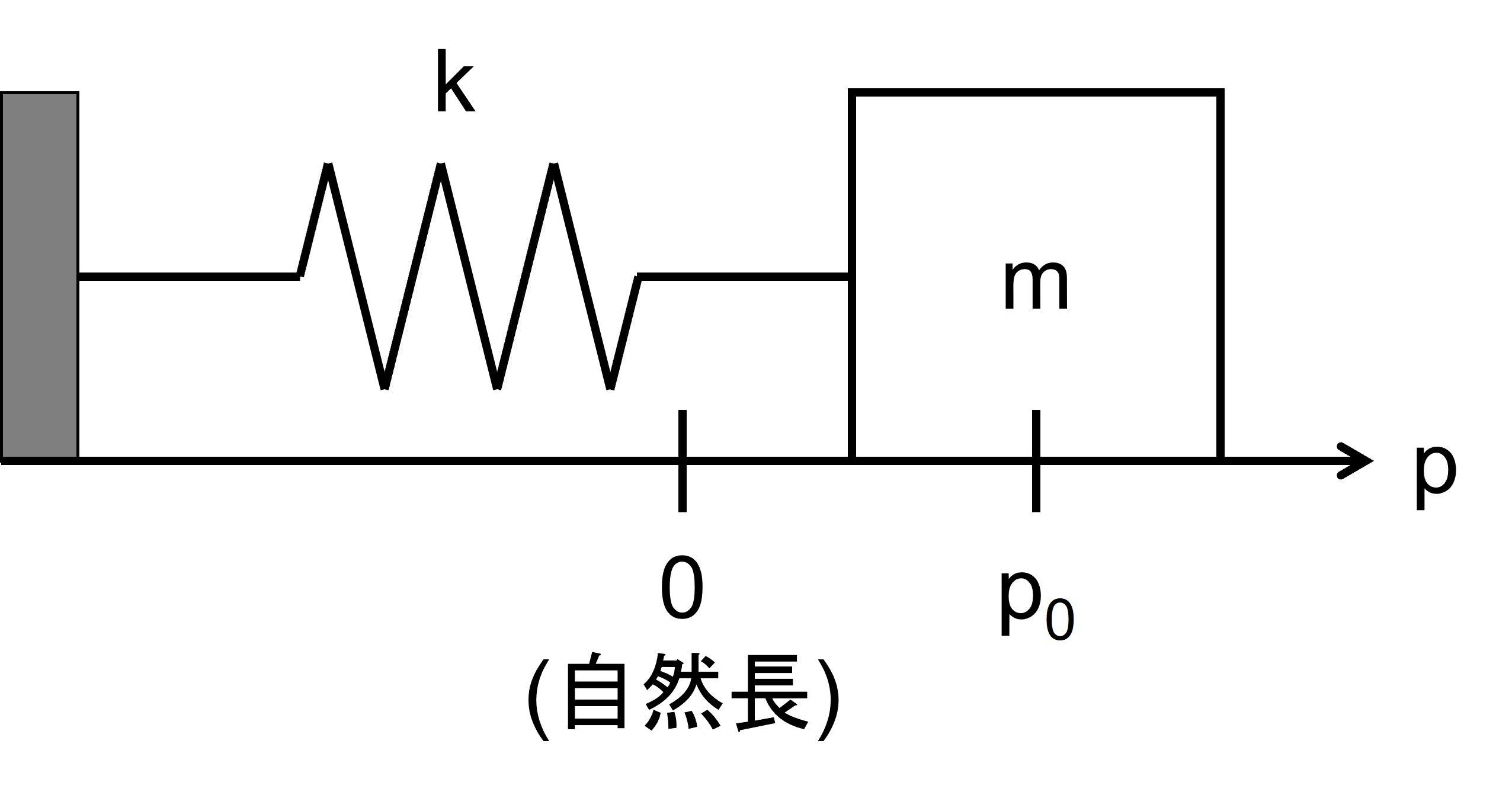
初期条件は以下
\begin{aligned}
p(0) &= p_0 \\
\dot{p}(0) &= 0
\end{aligned}
運動方程式は以下
\begin{aligned}
m\ddot{p}(t) = -kp(t)
\end{aligned}
シミュレーションには必要ではないが、今回のシステムは解析解が得られるので計算しておく。解析解は以下のようになる。
\begin{aligned}
p(t) &= p_0 \cos \sqrt{\frac{k}{m}}t \\
\dot{p}(t) &= -p_0 \sqrt{\frac{k}{m}}t \sin \sqrt{\frac{k}{m}}t
\end{aligned}
常微分方程式をつくる
運動方程式より、常微分方程式が以下のように書ける
\begin{aligned}
\dot{x}(t) &= f(x, t) \\
x(t) &=
\begin{bmatrix}
p(t) \\
\dot{p}(t) \\
\end{bmatrix} \\
f(x) &=
\begin{bmatrix}
0 & 1 \\
-\frac{k}{m} & 0 \\
\end{bmatrix}
x(t) \\
\end{aligned}
数値解法を用いてシミュレーションを行う
Euler法とRunge-Kutta法でシミュレーションした。
そのとき、タイムステップの長さを変え、シミュレーションの結果を厳密解と比較してみた。($\Delta t = 0.001, 0.01, 0.1, 1 (s)$)
システムのパラメタおよび初期値は以下で設定した。
\begin{aligned}
m &= 1 \\
k &= 2 \\
p_0 &= 1 \\
\end{aligned}
import numpy as np
import matplotlib.pyplot as plt

# set parameter
k = 2
m = 1

# define function
def ff(x):
    A = np.array([[0, 1], [-k/m, 0]])
    return A @ x

# Euler Method
def solve_ode_euler(x_old, func, dt):
    x_new = x_old + dt * func(x_old)
    return x_new

# Runge-Kutta Method
def solve_ode_rungekutta(x_old, func, dt):
    k1 = dt * func(x_old)
    k2 = dt * func(x_old + k1 / 2)
    k3 = dt * func(x_old + k2 / 2)
    k4 = dt * func(x_old + k3)
    x_new = x_old + (k1 + 2 * k2 + 2 * k3 + k4) / 6
    return x_new

# set initial state
x0 = np.array([[1], [0]])

# set time of simulation
dt_list = [0.001, 0.01, 0.1, 1]
tt_list = []
x_euler_list = []
x_rungekutta_list = []
for dt in dt_list:
    tt = np.arange(0, 20 + dt, dt)

    # simulation
    # Euler Method
    x_euler = np.zeros([2, tt.shape[0]])
    x_euler[:] = np.nan
    x_euler[:, 0:1] = x0
    x_old = x0
    for i in range(1, tt.shape[0]):
        x_new = solve_ode_euler(x_old=x_old, func=ff, dt=dt)
        x_euler[:, i:i+1] = x_new
        x_old = x_new

    # Runge-Kutta Method
    x_rungekutta = np.zeros([2, tt.shape[0]])
    x_rungekutta[:] = np.nan
    x_euler[:, 0:1] = x0
    x_old = x0
    for i in range(1, tt.shape[0]):
        x_new = solve_ode_rungekutta(x_old=x_old, func=ff, dt=dt)
        x_rungekutta[:, i:i+1] = x_new
        x_old = x_new

    # contain
    tt_list.append(tt)
    x_euler_list.append(x_euler)
    x_rungekutta_list.append(x_rungekutta)

# get exact solution
tt_real = tt_list[0]
p = x0[0] * np.cos(np.sqrt(k/m) * tt_real)
pdot = -x0[0] * np.sqrt(k/m) * np.sin(np.sqrt(k/m) * tt_real)
x_real = np.vstack([p, pdot])

# plot
for i in range(len(tt_list)):
    tt = tt_list[i]
    x_euler = x_euler_list[i]
    x_rungekutta = x_rungekutta_list[i]

    fig = plt.figure()
    ax1 = fig.add_subplot(2, 1, 1)
    ax2 = fig.add_subplot(2, 1, 2, sharex=ax1)
    ax1.grid()
    ax2.grid()

    ax1.plot(tt_real, x_real[0, :], color='gray')
    ax1.plot(tt, x_euler[0, :], '--', color='blue')
    ax1.plot(tt, x_rungekutta[0, :], '--', color='red')

    ax2.plot(tt_real, x_real[1, :], color='gray')
    ax2.plot(tt, x_euler[1, :], '--', color='blue')
    ax2.plot(tt, x_rungekutta[1, :], '--', color='red')

    ax1.legend(
        ['Exact solution', 'Euler', 'Runge-Kutta'],
        loc='upper left')
    ax1.set_title('dt = {:.3f} s'.format(dt_list[i]))
    ax1.set_ylabel('Position (m)')
    ax1.set_ylim([-3, 3])

    ax2.set_xlabel('Time (s)')
    ax2.set_ylabel('Velocity (m/s)')
    ax2.set_ylim([-3, 3])
    ax1.set_xlim([tt[0], tt[-1]])

plt.show()


$dt = 0.001s$ではEuler法とRunge-Kutta法のどちらも厳密解に近い運動をシミュレーションできているが、ステップ幅を長くした$dt = 0.01s$ではEuler法が厳密解とは異なることが見て取れる。一方で、Runge-Kutta法では$dt = 0.1s$でも厳密解に近い運動をシミュレーションできている。
シミュレーションのステップ幅は細かい方が精度が良い一方で、細かくしすぎると計算量が増えるといった問題がある。
こういった実用上の問題を把握し、十分な精度を出しつつ現実的な時間で終わるシミュレーションを設計する必要がある。
最後に
本記事では常微分方程式から時系列のシミュレーションへの手順を簡潔にまとめた。シミュレーションは研究活動において実用的な技術であるから、ぜひ使いこなしたい。
参考
常微分方程式の数値解法についての解説は以下の本が分かりやすかった。
山﨑匡、五十嵐潤「はじめての神経回路シミュレーション」森北出版 (2021)
サポートページ:https://numericalbrain.org/snsbook/