はじめに
以前からベータ提供されていたGranite時系列データ分析モデル(Timeseries Forecasting API)が2025年2月、ついに正式に提供開始されました。
本記事ではGranite時系列データ分析モデルを使って、将来の電力使用量の予測をしていきます。
Granite時系列データ分析モデルとは?
IBMが提供するGraniteモデルシリーズのひとつで、時系列データに対応した基盤モデルです。時系列基盤モデルは言語に特化した大規模言語モデルと同様に、膨大な時系列データを用いて事前学習されています。従来の時系列予測モデルとは異なり、特定のタスクに特化せず幅広い時系列予測タスクに対応可能となっており、さらに少ないデータからでも精度の高い予測が可能となっています。
Granite時系列データ分析モデルは他社と比べて軽量なモデルとなっており、CPUのみでも実行可能です。
Graniteモデルはオープンなモデルであることが特長のひとつとなっており、このモデルも他のGraniteモデルと同様にモデルの情報やトレーニングデータを公開しています。
https://huggingface.co/ibm-granite/granite-timeseries-ttm-r2
環境準備
実施にあたって以下の記事とNotebookを参考にしました。
https://www.ibm.com/think/tutorials/time-series-api-watsonx-ai
環境はwatsonx.aiのNotebookで実行しました。Python3.11のランタイムを使用しています。
まず必要なライブラリのインストールします。
%pip install wget | tail -n 1
%pip install -U matplotlib | tail -n 1
%pip install -U ibm-watsonx-ai | tail -n 1
次にwatsonx.aiの接続情報の設定をします。URLはお使いのリージョンに合わせて変更ください。
import getpass
from ibm_watsonx_ai import Credentials

credentials = Credentials(
    url="https://us-south.ml.cloud.ibm.com",
    api_key=getpass.getpass("Please enter your watsonx.ai api key (hit enter): "),
)
from ibm_watsonx_ai import APIClient

client = APIClient(credentials)
import os

try:
    project_id = os.environ["PROJECT_ID"]
except KeyError:
    project_id = input("Please enter your project_id (hit enter): ")
以下を実行して、問題がなければ'SUCCESS'とでます。
client = APIClient(credentials)
client.set.default_project(WATSONX_PROJECT_ID)
データセットの準備
使用するデータセットは2015-2018年にスペインで収集された4年間の電力消費量とエネルギー生成データが1時間刻みで集計されたデータです。
簡潔にするためデータセットは欠損値がなく、無関係な列が削除されています。
filename = 'energy_dataset.csv'
base_url = 'https://github.com/IBM/watson-machine-learning-samples/raw/refs/heads/master/cloud/data/energy/'
if not os.path.isfile(filename): wget.download(base_url + filename)
df = pd.read_csv(filename)
df.tail()
データセットの最後の数行を見てみます。時間列には、各時間のタイムスタンプが表示されています。他の列には、さまざまなソースからのエネルギー生成、天気予報の詳細、および実際のエネルギー使用量 ( total_load_actual ) の数値データ型が表示されます。
この total_load_actual がターゲット列、つまり値を予測しようとしている列になります。Granite時系列モデルは多変量予測が可能なため、他のすべての列をモデルへの入力として使用し、予測に使用します。
次にデータセットをトレーニングデータとグランドトゥルースに分割します。グランドトゥルースと時系列モデルの予測値を比較して、モデルの精度を確認します。
Granite時系列モデルは512、1024、1536トークンの3つのコンテキスト長のモデルを提供しています。コンテキスト長はモデルが予測を行うときに考慮できるデータ量を示しています。
今回は512トークンの時系列モデル、ibm/granite-ttm-512-96-r2を使用します。これを実行するためにはモデルの入力として512行のデータセット(履歴)が必要です。
このデータセットには512行より多くの行が含まれているため、データセットの最後からグランドトゥルースを96行抽出、トレーニングデータを512行抽出して、予測に使用します。
timestamp_column = "time"
target_column = "total load actual"
context_length = 608
future_context = 96

# Only use the last `context_length` rows for prediction.
future_data = df.iloc[-future_context:,]
data = df.iloc[-context_length:-future_context,]
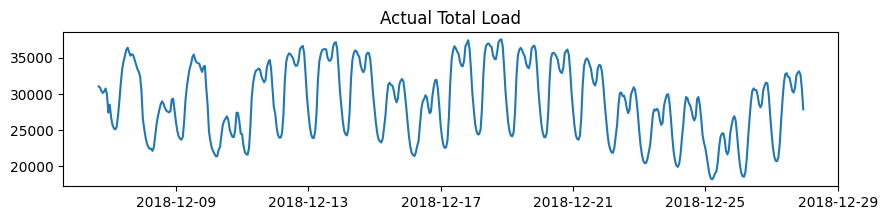
トレーニングデータを可視化します。
plt.figure(figsize=(10,2))
plt.plot(np.asarray(data[timestamp_column], 'datetime64[s]'), data[target_column])
plt.title("Actual Total Load")
plt.show()
watsonx.ai SDKのget_time_series_model_specs関数を使用すると、Timeseries Forecasting API から利用可能なモデルを一覧表示できます。
ここでは、512コンテキスト長のモデルを使用しますが、より大きなコンテキストモデルも利用できることがわかります。
for model in client.foundation_models.get_time_series_model_specs()["resources"]:
    print('--------------------------------------------------')
    print(f'model_id: {model["model_id"]}')
    print(f'functions: {model["functions"]}')
    print(f'long_description: {model["long_description"]}')
    print(f'label: {model["label"]}')
実行すると以下のアウトプットが出ます。
--------------------------------------------------
model_id: ibm/granite-ttm-1024-96-r2
functions: [{'id': 'time_series_forecast'}]
long_description: TinyTimeMixers (TTMs) are compact pre-trained models for Multivariate Time-Series Forecasting, open-sourced by IBM Research. Given the last 1024 time-points (i.e. context length), this model can forecast up to next 96 time-points (i.e. forecast length) in future. This model is targeted towards a forecasting setting of context length 1024 and forecast length 96 and recommended for hourly and minutely resolutions (Ex. 10 min, 15 min, 1 hour, etc)
label: granite-ttm-1024-96-r2
--------------------------------------------------
model_id: ibm/granite-ttm-1536-96-r2
functions: [{'id': 'time_series_forecast'}]
long_description: TinyTimeMixers (TTMs) are compact pre-trained models for Multivariate Time-Series Forecasting, open-sourced by IBM Research. Given the last 1536 time-points (i.e. context length), this model can forecast up to next 96 time-points (i.e. forecast length) in future. This model is targeted towards a forecasting setting of context length 1536 and forecast length 96 and recommended for hourly and minutely resolutions (Ex. 10 min, 15 min, 1 hour, etc)
label: granite-ttm-1536-96-r2
--------------------------------------------------
model_id: ibm/granite-ttm-512-96-r2
functions: [{'id': 'time_series_forecast'}]
long_description: TinyTimeMixers (TTMs) are compact pre-trained models for Multivariate Time-Series Forecasting, open-sourced by IBM Research. Given the last 512 time-points (i.e. context length), this model can forecast up to next 96 time-points (i.e. forecast length) in future. This model is targeted towards a forecasting setting of context length 512 and forecast length 96 and recommended for hourly and minutely resolutions (Ex. 10 min, 15 min, 1 hour, etc)
label: granite-ttm-512-96-r2
予測に使用するモデルを指定します。
ts_model_id = client.foundation_models.TimeSeriesModels.GRANITE_TTM_512_96_R2
TSModelInferenceクラスのオブジェクトを初期化します。
from ibm_watsonx_ai.foundation_models import TSModelInference

ts_model = TSModelInference(
    model_id=ts_model_id,
    api_client=client
)
モデルパラメータのセット、予測時間を1時間刻みに設定します。
from ibm_watsonx_ai.foundation_models.schema import TSForecastParameters

forecasting_params = TSForecastParameters(
    timestamp_column=timestamp_column,
    freq="1h",
    target_columns=[target_column],
)
forecast()メソッドを呼び出して、ターゲット変数total_load_actualの値を計算して、将来の電力使用量の予測する
results = ts_model.forecast(data=data, params=forecasting_params)['results'][0]
予測結果とグランドトゥルースを可視化します。
plt.figure(figsize=(10,2))
plt.plot(np.asarray(data[timestamp_column], dtype='datetime64[s]'), data[target_column], label="Historical data")
plt.plot(np.asarray(results[timestamp_column], dtype='datetime64[s]'), results[target_column], label="Predicted")
plt.plot(np.asarray(future_data[timestamp_column], dtype='datetime64[s]'), future_data[target_column], label="True", linestyle='dashed')
plt.legend(loc='center left', bbox_to_anchor=(1, 0.5))
plt.show()
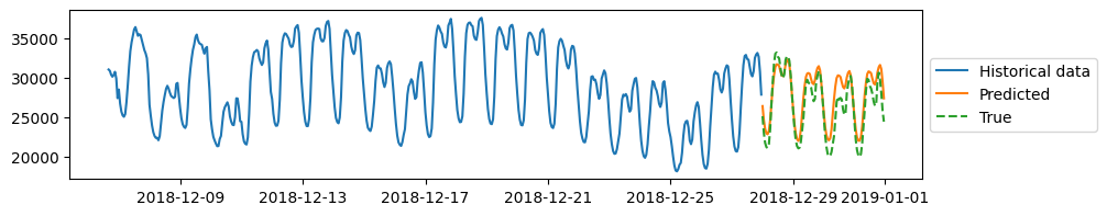
サンプルのノートブックにはありませんが、誤差を示すMAPEを導出します。
mape = mean_absolute_percentage_error(future_data[target_column], results[target_column]) * 100
mape
実行すると以下の結果となりました。このユースケースなら10%以下なら良い精度だそうなので、良い結果が出ていることがわかります。
6.081524040679701
まとめ
今回はファインチューニングなしのZero-Shotプロンプティングでの予測でしたので、あっという間に予測結果を出すことができ、さらにそれなりに高い精度で予測することができました。
今回は電力使用量の予測のユースケースで試してみましたが、株価の予測、排出量予測、業務効率化など様々なユースケースでGranite時系列予測モデルはお使いいただけます。ぜひ試してみてください。