この記事はR Advent Calendar 2018 15日目の記事です。
今回は、平成も終わるのでロバスト統計の話をしますね。(異論は受け付けない)
外れ値
何かしらの実験やデータを取った際に、分布を確認すると思います。
そんな時に、いくつかおかしなところにplotされてしまう何かがあるケース、よく出くわしますよね。
他のデータよりも明らかにおかしな値を取っているものを外れ値(Outlier)と言います。
具体的には下記のようなイメージです。
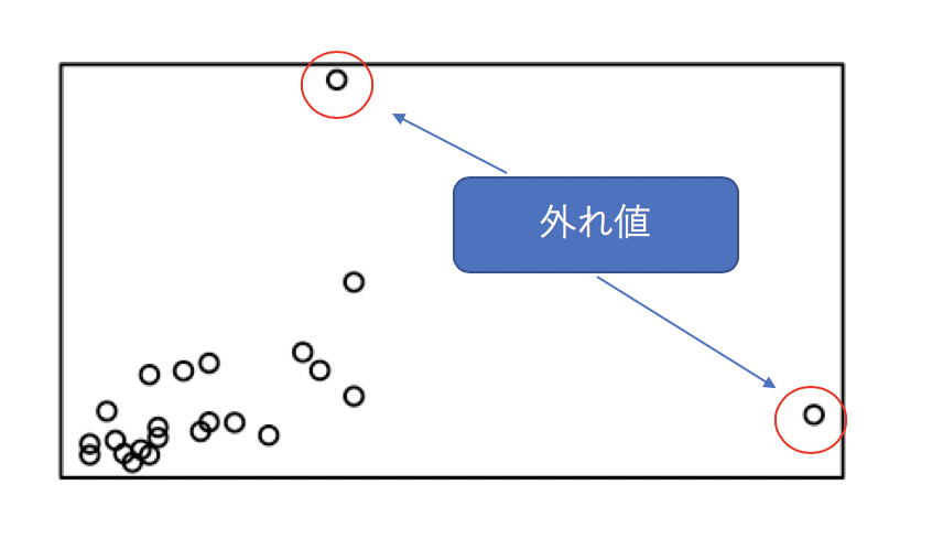
これを元に要約統計量などを算出しようとすると、外れ値の持つ値に引きずられて平均値などの代表値は信頼性を担保できなくなる可能性があります。
ロバスト統計とは
先ほど説明した外れ値の混入は未然に防ぐことができれば良いですね。しかし、データ取得の前に防げば良いのですが、なかなか思うようにうまくはいきません。サービスをリリースしたりすると、想定していなかった何かが起こることは日常茶飯事です。
そういう時には、外れ値などの混入を起こりうるものとして、対処する必要があります。
このように、外れ値が混入した場合でもメインとなる代表性を担保できるような統計モデルを組み立てたり、推定や検定を行うことをロバスト統計と言います。
何か外れ値が混入した時に、それを検知するモデルを作るようなアプローチをとると異常検知(Outlier Detection)となります。今回はこちらの話ではありません。
ロバストは日本語で訳すと頑健と言われます。
ロバストネスに関しては、ブラックスワンで有名なナシーム・ニコラス・タレブが著書の「On Robustness And Fragility」(邦訳:強さと脆さ)で取り上げたことでも有名です。

中央値
では、どう対処したら良いのでしょうか。結論から言うと、中央値を用いるのがベターです。
代表値の3つ。最頻値(mode)、平均値(mean)、中央値(median)の違いはWikipediaの下記の図がわかりやすいです。

このように平均では、分布が右に裾野を引いていると、その影響を受けてしまいやすく、中央値の場合は累積50%の値になるため、1つや2つの異常値が混入したとしても、それに引きづられることはありません。
M推定
ロバスト推定で最もポピュラーな手法です。
例えば、データX={x1,...xn}がある母集団からの標本だとします。
この母集団の分布を確率密度関数f(x:θ)とすると、最尤推定量は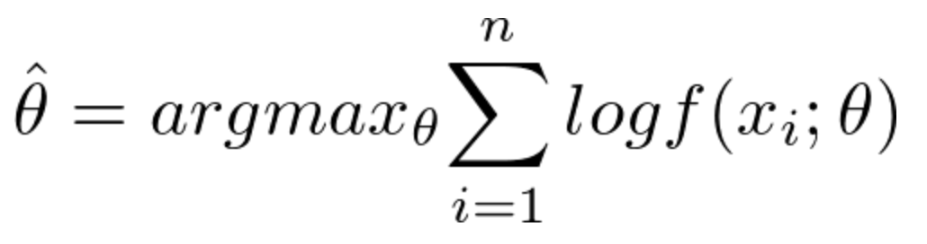
これを次のように書き換えます。
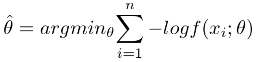
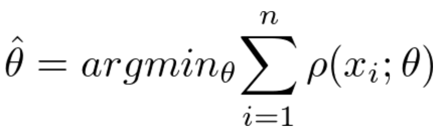
このようにすると、ロス関数を最小化する推定を行うことになります。これがM推定です。
一言で言えば、誤差があるデータに対してその誤差の影響を最小にするものです。
Rで使うには
{robustbase}パッケージにはかなり豊富にロバスト統計を行える関数が用意されています。
執筆時点でのCRANの最新情報だとアップデートも今年の9月に行われており、メンテナンスもされていそうです。
個人的にはこのパッケージ内に用意されているデータセットが豊富なことがテンションが上がるポイントでした。
データセット一覧
| Data | Description |
|---|---|
| Animals2 | Brain and Body Weights for 65 Species of Land Animals |
| CrohnD | Crohn's Disease Adverse Events Data |
| NOxEmissions | NOx Air Pollution Data |
| SiegelsEx | Siegel's Exact Fit Example Data |
| aircraft | Aircraft Data |
| airmay | Air Quality Data |
| alcohol | Alcohol Solubility in Water Data |
| ambientNOxCH | Daily Means of NOx (mono-nitrogen oxides) in air |
| biomassTill | Biomass Tillage Data |
| bushfire | Campbell Bushfire Data |
| carrots | Insect Damages on Carrots |
| cloud | Cloud point of a Liquid |
| coleman | Coleman Data Set |
| condroz | Condroz Data |
| cushny | Cushny and Peebles Prolongation of Sleep Data |
| delivery | Delivery Time Data |
| education | Education Expenditure Data |
| epilepsy | Epilepsy Attacks Data Set |
| exAM | Example Data of Antille and May - for Simple Regression |
| foodstamp | Food Stamp Program Participation |
| hbk | Hawkins Bradu Kass's Artificial Data |
| heart | Heart Catherization Data |
| kootenay | Waterflow Measurements of Kootenay River in Libby and Newgate |
| lactic | Lactic Acid Concentration Measurement Data |
| los | Length of Stay Data |
| milk | Daudin's Milk Composition Data |
| pension | Pension Funds Data |
| phosphor | Phosphorus Content Data |
| pilot | Pilot-Plant Data |
| possum.mat (possumDiv) | Possum Diversity Data |
| possumDiv | Possum Diversity Data |
| pulpfiber | Pulp Fiber and Paper Data |
| radarImage | Satellite Radar Image Data from near Munich |
| salinity | Salinity Data |
| starsCYG | Hertzsprung-Russell Diagram Data of Star Cluster CYG OB1 |
| steamUse | Steam Usage Data (Excerpt) |
| telef | Number of International Calls from Belgium |
| toxicity | Toxicity of Carboxylic Acids Data |
| vaso | Vaso Constriction Skin Data Set |
| wagnerGrowth | Wagner's Hannover Employment Growth Data |
| wood | Modified Data on Wood Specific Gravity |
データを眺める
こうなると、用意されているデータがどんな按配か確認したくなるのがRユーザーの性ですよね。
普通にpairs関数で散布図行列を描画しても良いのですが、せっかくなのでGGally::ggpairsで綺麗なplotを描いてみましょう
ggpairs(aircraft)

ggpairs(carrots)

ggpairs(milk)

ggpairs(wood)
 あー。いいですねぇ。ワクワクしますねぇ。
ロバスト回帰モデル
それでは、実際にパッケージに用意されているDatasetを使ってロバスト回帰を行ってみましょう。
一般的なロバスト回帰であるrobustbase::lmrobもありますが、なんとなく気分が乗らなかったので、一般化線形モデルベースのrobustbase::glmrobを使ってみます。
robustbase::glmrobは柔軟にモデリングができ、分布の指定はfamily = binomial, = poisson, = Gamma and = gaussianと4種類の選択が可能です。今回はbinomialを使います。
対象データはにんじんの損害データが記録されたrobustbase::data(carrots)を使います。
## robustbase
library(robustbase)

data(carrots)
Cfit1 <- glm(cbind(success, total-success) ~ logdose + block,
             data = carrots, family = binomial)
summary(Cfit1)
まずは普通にglmでやってみます。
Call:
glm(formula = cbind(success, total - success) ~ logdose + block,
    family = binomial, data = carrots)

Deviance Residuals:
    Min       1Q   Median       3Q      Max
-1.9200  -1.0215  -0.3239   1.0602   3.4324

Coefficients:
            Estimate Std. Error z value Pr(>|z|)
(Intercept)   2.0226     0.6501   3.111  0.00186 **
logdose      -1.8174     0.3439  -5.285 1.26e-07 ***
blockB2       0.3009     0.1991   1.511  0.13073
blockB3      -0.5424     0.2318  -2.340  0.01929 *
---
Signif. codes:  0 ‘***’ 0.001 ‘**’ 0.01 ‘*’ 0.05 ‘.’ 0.1 ‘ ’ 1

(Dispersion parameter for binomial family taken to be 1)

    Null deviance: 83.344  on 23  degrees of freedom
Residual deviance: 39.976  on 20  degrees of freedom
AIC: 128.61

Number of Fisher Scoring iterations: 4
Rfit1 <- glmrob(cbind(success, total-success) ~ logdose + block,
                family = binomial, data = carrots, method= "Mqle", #MrleはHuber Loss
                control= glmrobMqle.control(tcc=1.2))
summary(Rfit1)
Call:  glmrob(formula = cbind(success, total - success) ~ logdose +      block, family = binomial, data = carrots, method = "Mqle",      control = glmrobMqle.control(tcc = 1.2))


Coefficients:
            Estimate Std. Error z value Pr(>|z|)
(Intercept)   2.3883     0.6923   3.450 0.000561 ***
logdose      -2.0491     0.3685  -5.561 2.68e-08 ***
blockB2       0.2351     0.2122   1.108 0.267828
blockB3      -0.4496     0.2409  -1.866 0.061989 .
---
Signif. codes:  0 ‘***’ 0.001 ‘**’ 0.01 ‘*’ 0.05 ‘.’ 0.1 ‘ ’ 1
Robustness weights w.r * w.x:
 15 weights are ~= 1. The remaining 9 ones are
     2      5      6      7     13     14     21     22     23
0.7756 0.7026 0.6751 0.9295 0.8536 0.2626 0.8337 0.9051 0.9009

Number of observations: 24
Fitted by method ‘Mqle’  (in 9 iterations)

(Dispersion parameter for binomial family taken to be 1)

No deviance values available
Algorithmic parameters:
   acc    tcc
0.0001 1.2000
maxit
   50
test.acc
  "coef"
> coef(Cfit1)
(Intercept)     logdose     blockB2     blockB3
  2.0226453  -1.8174044   0.3008816  -0.5423898

> coef(Rfit1)
(Intercept)     logdose     blockB2     blockB3
  2.3882515  -2.0491078   0.2351038  -0.4496314
偏回帰係数の推定値の結果が異なっていますね。
(Intercept) と logdoseに関しては有意水準もかなり良さそうです。
一方で blockB3は精度が落ちてしまいました。
この辺りはきちんとしたデータ量を増やすことで解決できるかもしれませんね。
現場からは以上です。
Enjoy!
明日は Atsushi776さんです。楽しみですね。