🌾本記事は下記の環境に基づいて執筆されました
- macOS Mojave (ver. 10.14.6)
-- R (ver. 4.0.2)
--- tidyverse (ver. 1.3.0); dplyr (ver. 1.0.2); ggplot2 (ver. 3.3.2); patchwork (ver. 1.0.1)
🌾本記事の概要
# バイオ系wet研究者が
# Rを利用して
# 内在性トリプトファン蛍光消光試験のデータから
curve fittingにより結合パラメーターを決定する
はじめに
本記事はRあるいは各パッケージについて詳細に解説することを目的としていません。それらについては,他の多くの記事や書籍がとても丁寧に解説してくれています (他力本願)。
ただそれらの記事や書籍の多くは,irisやmpgのようなサンプルデータセットを利用して解説を行っており,自分 (特に蛋白質関係の測定/分析が専門) としては実用までの距離を感じて少しとっつきにくかったように思います。
そういった視点でネット上の解説記事を眺めてみると,実際の実験データを利用して解説している記事って案外少ないんじゃないかと思います。やっぱり実験データはおいそれと公開できないからですかね。
そこでこのシリーズでは,私が大学/大学院時代に測定したけどボツった実験データの中でも公開してなんら問題ないデータを活用して,研究の中で行ってきた解析を共有できたら良いなと考えています。
「ああ,こういう使い方もできるのね」という感じで,誰かの (特に自分と専門が近い人たちの) モチベーションにつながることがあれば,それはとっても嬉しいなって。
背景を少しばかり
蛋白質とリガンドとの相互作用解析
蛋白質とリガンド (結合パートナー分子) との相互作用は,生体内における様々な分子イベントに関与するギミックです。応用的には,例えば創薬研究において標的蛋白質と特異的に結合する阻害剤を探索する過程では,標的蛋白質のどこに阻害剤分子が結合するかとか標的蛋白質に対して阻害剤がどのくらいの結合親和性で結合するかを実験的に明らかにすることが重要だったりします (めっちゃざっくりですが……)。
蛋白質に対するリガンドの結合親和性を決定する実験手法はいくつも存在します。ここですべてを挙げることはしませんが,王道的にはsurface plasmon resonance (SPR) やisothermal titration calorimetry (ITC),そして最近流行ってきている (?) microscale thermophoresis (MST) あたりでしょうか。
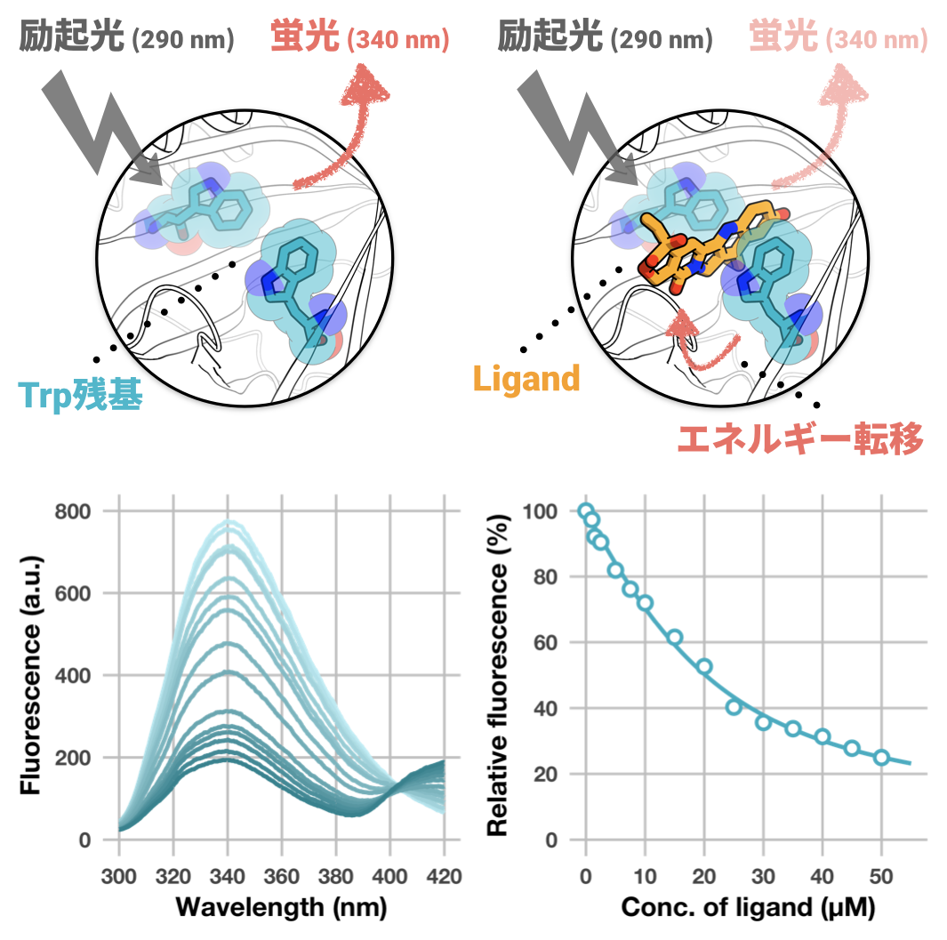
これらの手法はいずれも強力なのですが,いかんせんどれも高額な装置 (しかもそれほど汎用性がない) を必要とするため,研究環境によっては実施するのが難しいこともあるかもしれません。そこで今回は,比較的近場に転がっている (高額じゃないとは言っていない) 蛍光分光光度計を利用した内在性トリプトファン蛍光消光試験 (intrinsic tryptophan fluorescence quenching assay) を紹介したいと思います。
内在性トリプトファン蛍光消光試験
蛋白質の蛍光は,蛋白質に含まれる芳香族アミノ酸残基 (トリプトファン,チロシン,フェニルアラニン) に由来しますが,その中でもトリプトファン残基の寄与が非常に強いことが知られています (特に波長290 nmで励起光を用いた場合)。
この内在性トリプトファン残基に由来する蛍光強度は,トリプトファン残基インドール環周辺の化学環境に強く影響されます。例えば,リガンド分子が蛋白質のトリプトファン残基近傍に結合した場合,本来蛍光として放出されるエネルギーがリガンドに転移して蛍光強度が減少することがあります。この現象は,リガンド結合に伴う蛍光消光と表現されます。

つまり,添加するリガンド濃度を変化させて蛋白質 (濃度一定) の蛍光強度を測定 (いわゆる滴定実験) することにより,結合反応に伴う蛍光消光をモニターすることができます。さらに,実験結果に対してone-set of independent binding sites model (詳しくは記事末のAppendixを参照) を用いた非線形回帰分析を行うことで,蛋白質に対するリガンドの結合親和性 (具体的には解離定数 [ $K_\mathrm{d}$ ]) を決定することができます。
あと,本試験の良いところはもう一つありまして,原理上リガンドの結合位置に関する情報が得られます (これはSPR,ITC,およびMSTにはない利点です)。どんな結合配座かまでは明らかにできませんが,リガンド濃度依存的な蛍光消光が観察された場合,トリプトファン残基近傍にリガンドが結合したと考察することは可能でしょう。弱点としては,そもそもトリプトファン残基を有していない蛋白質は測定できないし,複数トリプトファン残基がある場合は解釈がややこしくなることがある,というところでしょうか。
本記事では,実際の内在性トリプトファン蛍光消光試験の実験データを用いて,Rを利用した非線形回帰分析 (curve fitting) による結合親和性の決定方法を紹介したいと思います。
実験データについて
今回用いる実験データをGoogleスプレッドシートにアップしました
https://docs.google.com/spreadsheets/d/16ywcmf8yKa29oLTRN4vMekKsCloE4nfjNDOl8wQfT0U/edit?usp=sharing
本データの内容は,某リガンド (低分子化合物) 濃度を変化させたときの某蛋白質 (5 μM) の蛍光スペクトル (excitation:290 nm)です。
wavelength_nm:測定波長 (nm)
ligand_*uM:各リガンド濃度 (μM) におけるwavelength_nm列に対する蛍光強度 (a. u.)
測定温度は37°C,測定bufferは5% (v/v) DMSOを含むPBS (pH 7.4) です。リガンドが難水溶性であるためDMSOが含まれています。
また,本蛍光スペクトルは,蛍光分光光度計F-7000 (Hitachi) を用いて測定されました。
以降はこのデータがquench.xlsxのquenchシートに記録されているものとして説明を行います。
実験データの解析
必要なパッケージの準備
それでは早速解析を行っていきます。
はじめに必要なパッケージのインストールと読み込みを行います。
# パッケージのインストール
install.packages("tidyverse")
install.packages("patchwork")

# パッケージの読み込み
library(tidyverse)
library(readxl)
library(patchwork)
tidyverseには今後使用する様々なパッケージ (例えばdplyrやggplot2など) が含まれています。
readxlはExcelファイルを読み込むために使用します。
readxlはtidyverseに含まれているため個別でのインストールは不要ですが,使用するためには個別に読み込む必要があります。
patchworkは複数のグラフを一つのfigureにまとめる際に利用します。
測定データのインポート & データ整形
Excelファイルにまとめた測定データquench.xlsxをインポートしてquench_rawに格納します。
# 測定データをExcelファイルからインポート
quench_raw <- read_excel("quench.xlsx", sheet = "quench")
quench_rawの中身はこんな感じです。いい感じに読み込めていますね。
> quench_raw
# A tibble: 601 x 16
   wavelength_nm ligand_0uM ligand_1uM ligand_1.5uM ligand_2.5uM ligand_5uM ligand_7.5uM ligand_10uM ligand_15uM
           <dbl>      <dbl>      <dbl>        <dbl>        <dbl>      <dbl>        <dbl>       <dbl>       <dbl>
 1          300        43.6       44.7         46.1         46.0       43.2         38.6        37.4        35.1
 2          300.       43.9       44.7         46.5         46.0       42.9         38.5        38.0        35.4
 3          300.       44.3       45.4         46.9         46.1       43.7         39.3        38.8        36.4
 4          301.       45.2       46.1         47.8         46.6       44.2         40.2        39.5        36.7
 5          301.       47.3       47.5         48.4         47.4       45.3         40.8        40.1        37.6
 6          301        48.7       48.8         49.8         48.7       46.1         42.0        41          38.2
 7          301.       49.5       50.1         50.8         49.9       47.3         43.1        42.5        39.2
 8          301.       50.5       51.8         53.1         51.2       48.4         44.1        43.1        40.3
 9          302.       52.4       53.9         54.9         53.0       50.1         45.7        44.5        41.4
10          302.       54.4       55.8         56.7         54.9       51.9         47.1        45.9        42.6
# … with 591 more rows, and 7 more variables: ligand_20uM <dbl>, ligand_25uM <dbl>, ligand_30uM <dbl>,
#   ligand_35uM <dbl>, ligand_40uM <dbl>, ligand_45uM <dbl>, ligand_50uM <dbl>
続いて,dplyr::pivot_longer()関数を利用して,quench_rawをtidy dataに変換します。
# 実験データをtidy dataに変換
quench <- quench_raw %>%
  pivot_longer(cols = -wavelength_nm, names_to = "conc_uM", values_to = "fluoresc")
quenchの中身はこんな感じです。
> quench
# A tibble: 9,015 x 3
   wavelength_nm conc_uM      fluoresc
           <dbl> <chr>           <dbl>
 1           300 ligand_0uM       43.6
 2           300 ligand_1uM       44.7
 3           300 ligand_1.5uM     46.1
 4           300 ligand_2.5uM     46.0
 5           300 ligand_5uM       43.2
 6           300 ligand_7.5uM     38.6
 7           300 ligand_10uM      37.4
 8           300 ligand_15uM      35.1
 9           300 ligand_20uM      31.7
10           300 ligand_25uM      29.5
# … with 9,005 more rows
これでtidy dataに変換できましたが,以降のことを考えて形式をもう少し整えます。
具体的には,conc_uM列を濃度の値に置換 (例:ligand_5uM → 5) した後,conc_uMを基準にデータをソートします。
この操作,前回の記事では下記のようにゴリ押していました……。
# 実験データをtidy dataに変換
quench <- quench_raw %>%
  pivot_longer(cols = -wavelength_nm, names_to = "conc_uM", values_to = "fluoresc") %>%
  mutate(conc_uM = case_when(
    str_detect(conc_uM, fixed("_0uM")) ~ 0,
    str_detect(conc_uM, fixed("_1uM")) ~ 1,
    str_detect(conc_uM, fixed("_1.5uM")) ~ 1.5,
    str_detect(conc_uM, fixed("_2.5uM")) ~ 2.5,
    str_detect(conc_uM, fixed("_5uM")) ~ 5,
    str_detect(conc_uM, fixed("_7.5uM")) ~ 7.5,
    str_detect(conc_uM, fixed("_10uM")) ~ 10,
    str_detect(conc_uM, fixed("_15uM")) ~ 15,
    str_detect(conc_uM, fixed("_20uM")) ~ 20,
    str_detect(conc_uM, fixed("_25uM")) ~ 25,
    str_detect(conc_uM, fixed("_30uM")) ~ 30,
    str_detect(conc_uM, fixed("_35uM")) ~ 35,
    str_detect(conc_uM, fixed("_40uM")) ~ 40,
    str_detect(conc_uM, fixed("_45uM")) ~ 45,
    str_detect(conc_uM, fixed("_50uM")) ~ 50)) %>%
  select(conc_uM, wavelength_nm, fluoresc) %>%
  arrange(conc_uM)
我ながら酷い……。
というわけで,こんなときはreadr::parse_number()関数を利用して数字部分だけを抜き出してやりましょう。
# 実験データをtidy dataに変換
quench <- quench_raw %>%
  pivot_longer(cols = -wavelength_nm, names_to = "conc_uM", values_to = "fluoresc") %>%
  mutate(conc_uM = parse_number(conc_uM)) %>%   # conc_uM列を編集
  select(conc_uM, wavelength_nm, fluoresc) %>%  # 列の並びを編集
  arrange(conc_uM)                              # conc_uM列を基準にソート
するとquenchの中身はこうなります。いい感じに整理できましたね。
> quench
# A tibble: 9,015 x 3
   conc_uM wavelength_nm fluoresc
     <dbl>         <dbl>    <dbl>
 1       0          300      43.6
 2       0          300.     43.9
 3       0          300.     44.3
 4       0          301.     45.2
 5       0          301.     47.3
 6       0          301      48.7
 7       0          301.     49.5
 8       0          301.     50.5
 9       0          302.     52.4
10       0          302.     54.4
# … with 9,005 more rows
蛍光スペクトルをプロット
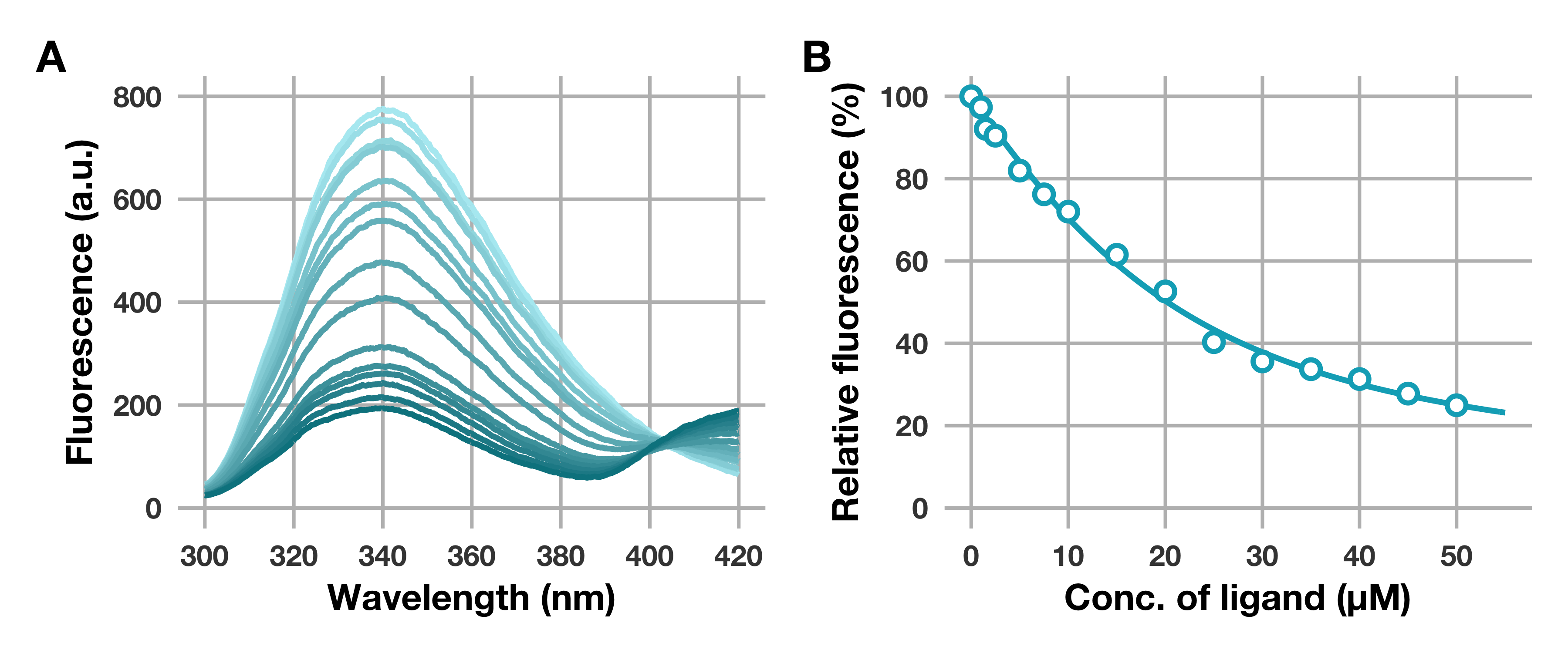
ひとまずデータの整形が終わったので,次に各リガンド濃度における蛍光スペクトルをプロットしてみましょう。
まずはグラフのテーマを設定します (macOSとWindowsで一部異なります)。
# グラフのテーマ設定 (macOSの場合)
theme_set(
  theme_minimal(base_size = 20, base_family = "Helvetica Neue Bold") +
  theme(
    panel.grid.major = element_line(colour = "#BDBDBD"),
    panel.grid.minor = element_blank(),
    axis.title.x = element_text(margin = margin(7, 0, 0, 0)),
    axis.title.y = element_text(margin = margin(0, 8, 0, 0)),
    axis.text = element_text(colour = "#424242"),
    plot.background = element_rect(fill = "transparent", colour = NA),
    legend.title = element_blank(),
    legend.justification = "top"
  )
)

# グラフのテーマ設定 (Windowsの場合)
windowsFonts(SG = windowsFont("Segoe UI Bold"))        # この行が違う
theme_set(
  theme_minimal(base_size = 20, base_family = "SG") +  # この行も少し違う
  theme(
    panel.grid.major = element_line(colour = "#BDBDBD"),
    panel.grid.minor = element_blank(),
    axis.title.x = element_text(margin = margin(7, 0, 0, 0)),
    axis.title.y = element_text(margin = margin(0, 8, 0, 0)),
    axis.text = element_text(colour = "#424242"),
    plot.background = element_rect(fill = "transparent", colour = NA),
    legend.title = element_blank(),
    legend.justification = "top"
  )
)
それではggplot2を用いて蛍光スペクトルをプロットします。
# 蛍光スペクトルをプロット
g_quench_spe <- quench %>%
  ggplot(mapping = aes(x = wavelength_nm, y = fluoresc, group = conc_uM, colour = conc_uM)) +
  geom_line(size = 1.5) +
  scale_colour_gradient(low = "#B2EBF2", high = "#00838F") +              # conc_uMの値を基準にグラジエント
  scale_x_continuous(breaks = seq(300, 420, 20), limits = c(300, 420)) +  # x軸のレンジ
  scale_y_continuous(breaks = seq(0, 800, 200), limits = c(0, 800)) +     # y軸のレンジ
  labs(x = "Wavelength (nm)", y = "Fluorescence (a.u.)") +                # x, y軸のラベル
  theme(legend.position = "none")                                         # レジェンドを表示しない
こんな感じのグラフが出力されます。
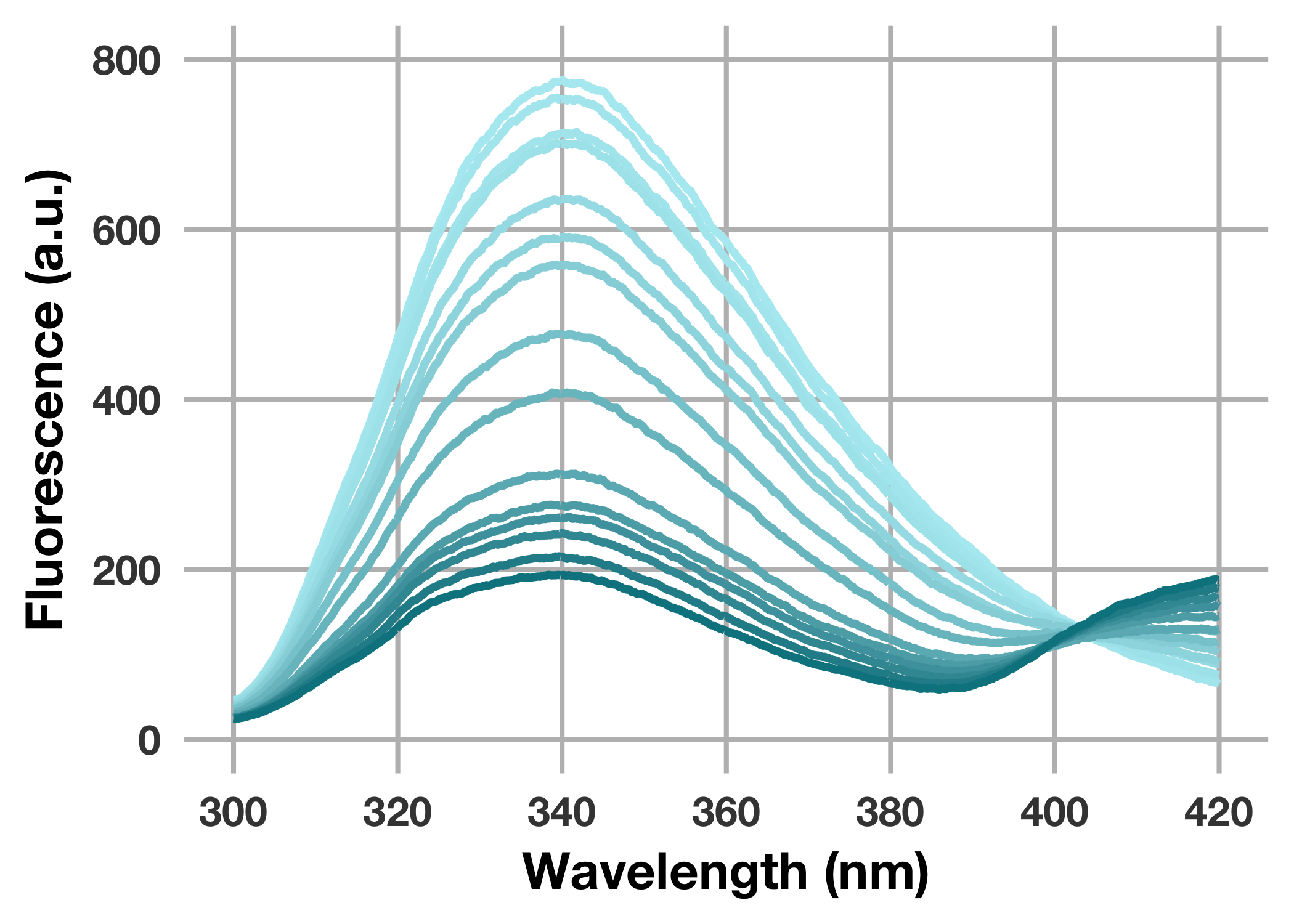
一見うまくプロットできたように見えますが,実はグラジエントのかけ方に問題 (?) があります。等間隔でないconc_uMの値を基準にグラジエントをかけているためです (今回はスペクトル毎に均等にグラジエントをかけたい)。そこで一工夫加えます。
# 蛍光スペクトルをプロット (改)
g_quench_spe <- quench %>%
  mutate(colour_steps = group_indices(., conc_uM)) %>%
  ggplot(mapping = aes(x = wavelength_nm, y = fluoresc, group = colour_steps, colour = colour_steps)) +
  geom_line(size = 1.5) +
  scale_colour_gradient(low = "#B2EBF2", high = "#00838F") +              # colour_stepsの値を基準にグラジエント
  scale_x_continuous(breaks = seq(300, 420, 20), limits = c(300, 420)) +  # x軸のレンジ
  scale_y_continuous(breaks = seq(0, 800, 200), limits = c(0, 800)) +     # y軸のレンジ
  labs(x = "Wavelength (nm)", y = "Fluorescence (a.u.)") +                # x, y軸のラベル
  theme(legend.position = "none")                                         # レジェンドを表示しない
mutate(colour_steps = group_indices(., conc_uM))で一時的にcolour_steps列を追加しています。
(dplyr::group_indices()関数によって,conc_uMの値毎に数字1, 2, 3, ...を割り当てています)
また,ggplot2::ggplot()関数中のgroupとcolourにそれぞれcolour_stepsを指定することで,colour_stepsの値に基づいてグラジエントをかけています。
できあがるグラフはこんな感じです。
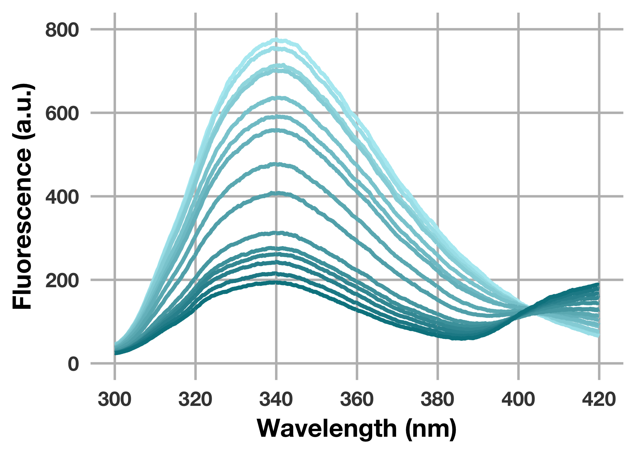
リガンド濃度依存的に (青色が濃くなる毎に) 波長340 nm付近の蛍光強度が減少していることが示されました。
リガンド濃度に対してピークトップの相対蛍光強度をプロット
リガンド濃度依存的な蛍光強度の変化を明確に示すために,リガンド濃度に対してピークトップの相対蛍光強度をプロットしてみましょう。
次のようにピークトップの蛍光強度を抽出し,リガンド非存在下の蛍光強度を100%とした際の相対蛍光強度を求めます。
# ピークトップにおける蛍光強度の抽出と相対蛍光強度の算出
quench_peak <- quench %>%
  group_by(conc_uM) %>%                                                   # conc_uMでグループ化
  summarise(fluoresc_peak = max(fluoresc)) %>%                            # ピークトップの蛍光強度を抽出
  mutate(relative_fluoresc = fluoresc_peak / first(fluoresc_peak) * 100)  # 相対蛍光強度の算出
conc_uMでグループ化してからdplyr::summarise()関数を使用することで,conc_uMの値毎に最大値を抽出することができます。
quench_peakの中身はこんな感じ。
> quench_peak
# A tibble: 15 x 3
   conc_uM fluoresc_peak relative_fluoresc
     <dbl>        <dbl>             <dbl>
 1     0           776.             100
 2     1           755.              97.3
 3     1.5         715.              92.1
 4     2.5         702.              90.4
 5     5           636               81.9
 6     7.5         591.              76.2
 7    10           559.              72.0
 8    15           477.              61.5
 9    20           408.              52.6
10    25           313.              40.3
11    30           276.              35.6
12    35           262.              33.7
13    40           243.              31.3
14    45           216.              27.8
15    50           194.              25.0
リガンド濃度conc_uMに対して相対蛍光強度relative_fluorescをプロットします。
# リガンド濃度に対して相対蛍光強度をプロット
g_quench_peak <- quench_peak %>%
  ggplot(mapping = aes(x = conc_uM, y = relative_fluoresc)) +
  geom_point(shape = 21, colour = "#00ACC1", fill = "white", size = 3.5, stroke = 2) +
  scale_x_continuous(breaks = seq(0, 50, 10), limits = c(0, 55)) +     # x軸のレンジ
  scale_y_continuous(breaks = seq(0, 100, 20), limits = c(0, 100)) +   # y軸のレンジ
  labs(x = "Conc. of ligand (μM)", y = "Relative fluorescence (%)") +  # x, y軸のラベル
  theme(legend.position = "none")                                      # レジェンドを表示しない
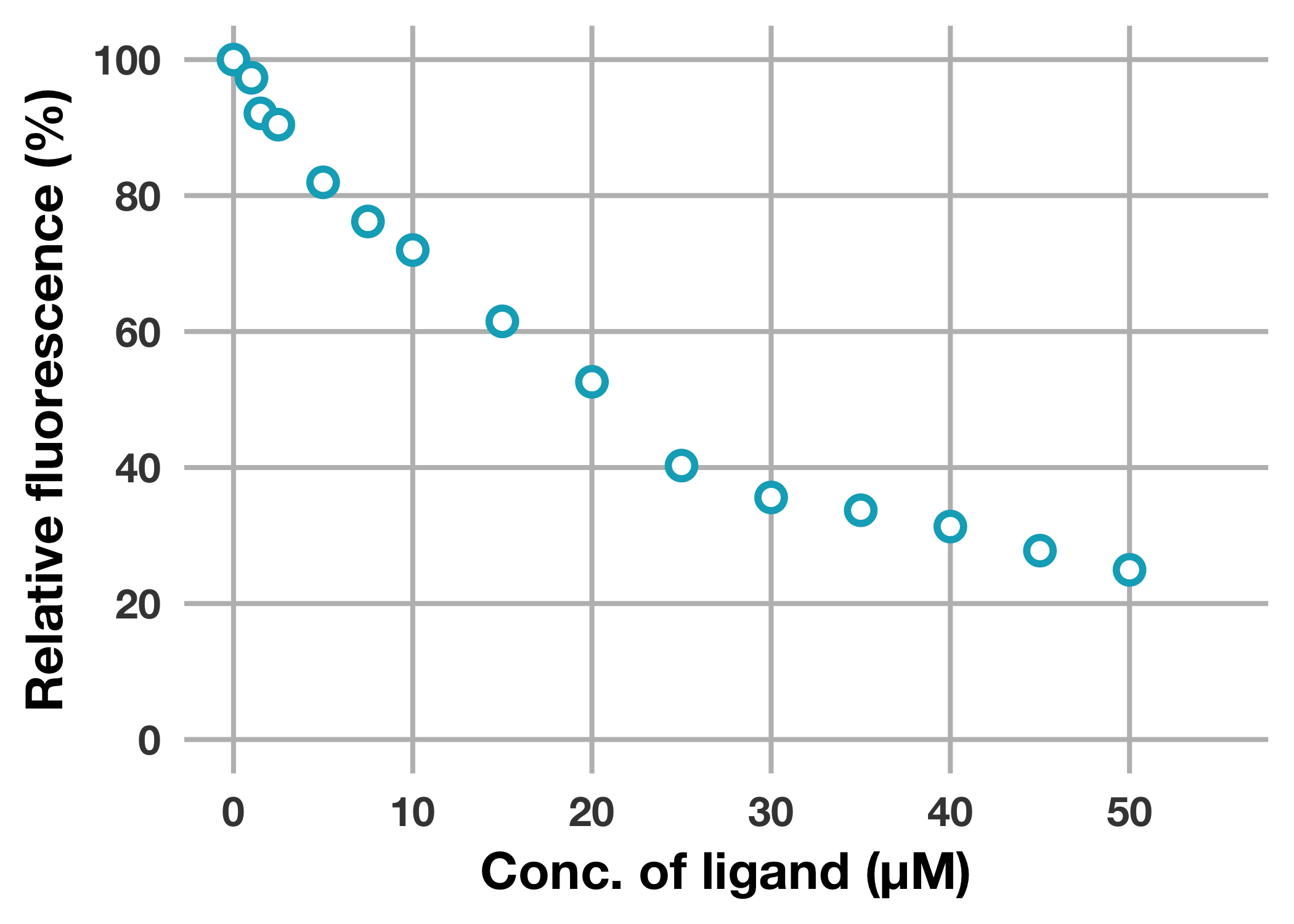
リガンド濃度依存的な蛍光消光を明確に示すことができました。
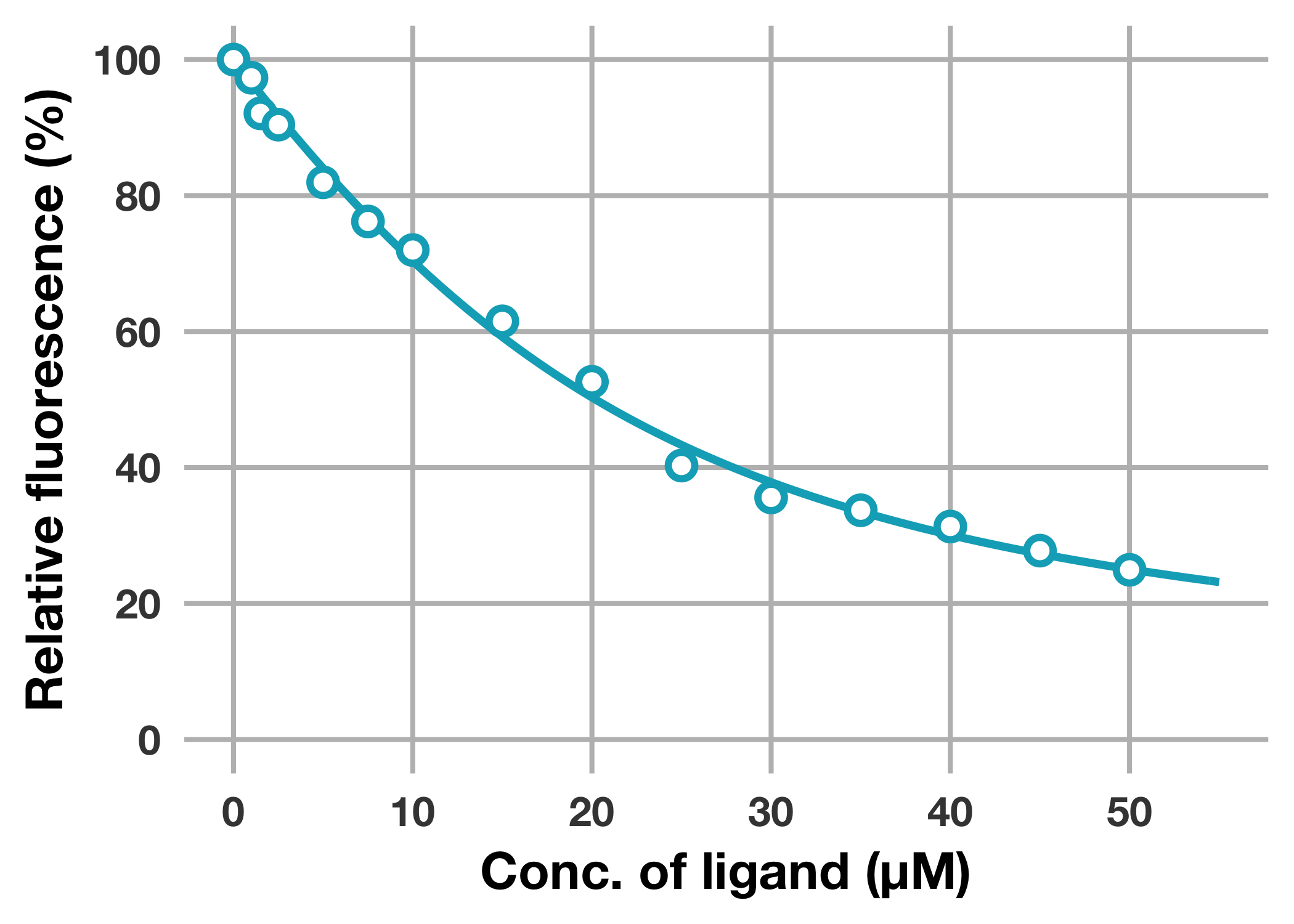
Curve fittingによる結合パラメーターの決定
最後に,リガンド濃度に対する相対蛍光強度変化のデータに対して,代表的な蛋白質–リガンド相互作用モデルであるone-set of independent binding sites modelに基づく下記の式を用いたcurve fittingを実施し,解離定数 ( $K_\mathrm{d}$ ) および結合数 ( $n$ ) を決定します。
\begin{align}
F &= \frac{n \mathrm{[P_0]} - \mathrm{[L_0]} - K_\mathrm{d}
            + \sqrt{(\mathrm{[L_0]} - n \mathrm{[P_0]} + K_\mathrm{d})^2 + 4n \mathrm{[P_0]} K_\mathrm{d}}}
          {2n \mathrm{[P_0]}} \times (F_{\mathrm{P}} - F_{\mathrm{PL}})
     + F_\mathrm{PL} \\
\end{align}
ここで,$F$,$F_\mathrm{P}$,および $F_\mathrm{PL}$ は,それぞれ測定により得られた蛍光強度,遊離状態 (リガンド非結合状態) における蛋白質の蛍光強度,およびリガンド結合状態における蛋白質の蛍光強度を表しています。
また,$\mathrm{[P_0]}$ および $\mathrm{[L_0]}$ は,それぞれ総蛋白質濃度 (遊離状態 & リガンド結合状態) および総リガンド濃度 (遊離状態 & 蛋白質結合状態) を表しています。
式の導出については記事末のAppendixを参照ください。
まず,fitting関数fun_Kd()を定義します。
# fitting関数を定義
fun_Kd <- function(L, P, n, Kd, F_p, F_pl) {
  b <- L - n * P + Kd
  return((- b + sqrt(b^2 + 4 * n * P * Kd)) * (F_p - F_pl) / (2 * n * P) + F_pl)
}
次に,定義したfun_Kd()関数とstats::nls()関数を用いてcurve fittingを実施し,fitting結果をfit_Kdに格納します。
# curve fitting
fit_Kd <- quench_peak %>%
  nls(
    relative_fluoresc ~ fun_Kd(L = conc_uM, P = 5, n, Kd, F_p = 100, F_pl),
    data = .,
    algorithm = "port",                       # lowerを指定するため
    start = list(n = 1, Kd = 10, F_pl = 20),  # 初期値の設定
    lower = list(F_pl = 0)                    # F_pl ≥ 0
  )
base::summary()関数を用いてfitting結果を確認します。
> summary(fit_Kd)

Formula: relative_fluoresc ~ fun_Kd(L = conc_uM, P = 5, n, Kd, F_0 = 100, F_min)

Parameters:
      Estimate Std. Error t value Pr(>|t|)
n       3.6270     0.9539   3.802  0.00252 **
Kd      9.6541     5.3936   1.790  0.09871 .
F_min   4.7885     9.8952   0.484  0.63715
---
Signif. codes:  0 ‘***’ 0.001 ‘**’ 0.01 ‘*’ 0.05 ‘.’ 0.1 ‘ ’ 1

Residual standard error: 1.915 on 12 degrees of freedom

Algorithm "port", convergence message: relative convergence (4)
$n$ および $K_\mathrm{d}$ は,それぞれ3.6 ± 0.95および9.7 ± 5.4 μMと求まりました。
それでは決定したパラメーターから得られるfitting curveをさきほどのプロットに重ねてみましょう。
fitting curveの描画にはggplot2:stat_function()関数を利用します。
# fitting curveを重ね書きする
g_fit_Kd <- quench_peak %>%
  ggplot(mapping = aes(x = conc_uM, y = relative_fluoresc)) +
  stat_function(
    fun = fun_Kd,                                           # 関数の指定
    args = list(P = 5,                                      # パラメーターの指定
                n = coef(fit_Kd)[1], Kd = coef(fit_Kd)[2],
                F_p = 100, F_pl = coef(fit_Kd)[3]),
    colour = "#00ACC1", size = 1.5) +
  geom_point(shape = 21, colour = "#00ACC1", fill = "white", size = 3.5, stroke = 2) +
  scale_x_continuous(breaks = seq(0, 50, 10), limits = c(0, 55)) +     # x軸のレンジ
  scale_y_continuous(breaks = seq(0, 100, 20), limits = c(0, 100)) +   # y軸のレンジ
  labs(x = "Conc. of ligand (μM)", y = "Relative fluorescence (%)") +  # x, y軸のラベル
  theme(legend.position = "none")                                      # レジェンドを表示しない
fitting curveをプロットに重ねることができました。
せっかくなのでpatchworkライブラリーを使ってスペクトルのプロットと並べて出力してみましょう。
(g_spe | g_fit_Kd) + plot_annotation(tag_levels = "A")
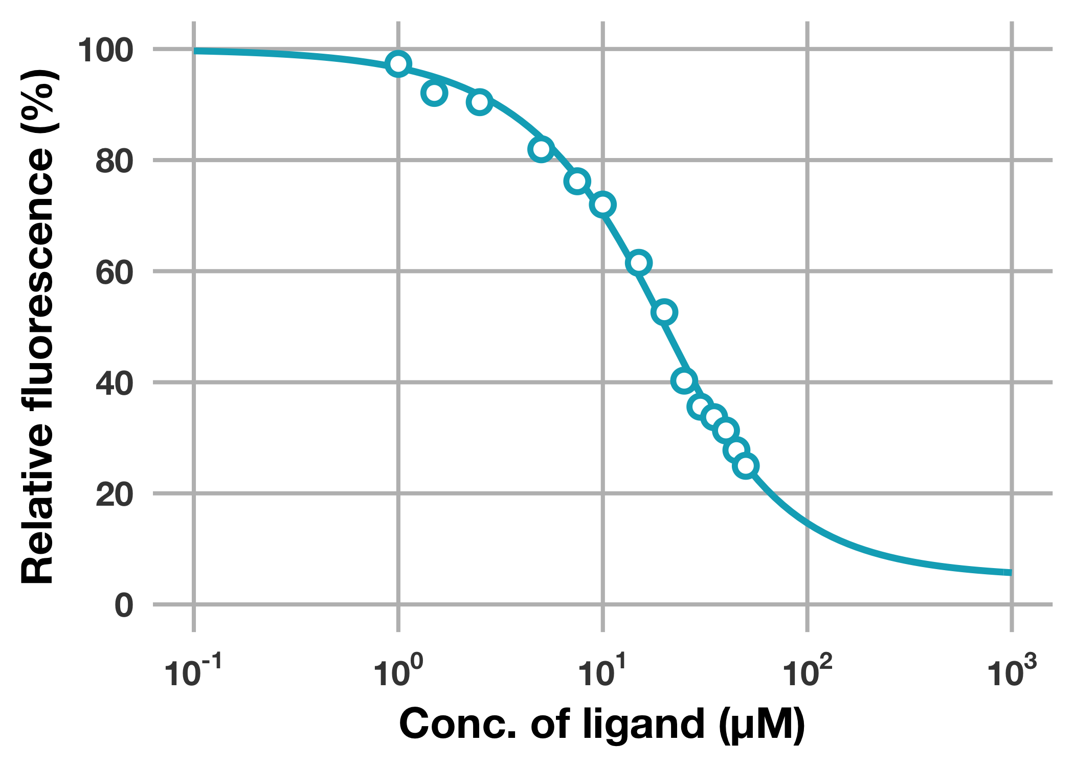
これは余談ですが,もう少し精度良く結合パラメーターを決定するためには,より高濃度域のデータを取る必要がありそうです (今回のリガンドは難水溶性化合物なので,実験的に無理なんですけどね)。
同様のプロットをlogスケールで表示すると高濃度域のデータが足りていないことがよくわかります。
# fitting curveを重ね書きする (logスケール)
g_fit_Kd_log <- quench_peak %>%
  filter(conc_uM > 0) %>%
  ggplot(mapping = aes(x = conc_uM, y = relative_fluoresc)) +
  stat_function(
    fun = fun_Kd,                                           # 関数の指定
    args = list(P = 5,                                      # パラメーターの指定
                n = coef(fit_Kd)[1], Kd = coef(fit_Kd)[2],
                F_p = 100, F_pl = coef(fit_Kd)[3]),
    colour = "#00ACC1", size = 1.5) +
  geom_point(shape = 21, colour = "#00ACC1", fill = "white", size = 3.5, stroke = 2) +
  scale_x_log10(                                                           # x軸をlogスケールに変換
    breaks = 10^(-1:3), limits = c(0.1, 1000),                             # x軸のレンジ
    labels = scales::trans_format("log10", scales::math_format(10^.x))) +  # x軸の数字表示を10^形式に
  scale_y_continuous(breaks = seq(0, 100, 20), limits = c(0, 100)) +       # y軸のレンジ
  labs(x = "Conc. of ligand (μM)", y = "Relative fluorescence (%)") +      # x, y軸のラベル
  theme(legend.position = "none")                                          # レジェンドを表示しない
以上で蛍光消光試験の解析は完了です!
次回予告
次回は蛋白質熱変性試験の解析を予定しています (論文がアクセプトされたら……)。
Appendix: One-set of independent binding sites model
もっともシンプルな蛋白質 ( $\mathrm{P}$ ) とリガンド ( $\mathrm{L}$ ) との1:1結合モデルは,次のように表されます。
\begin{align}
&\mathrm{P} + \mathrm{L} \rightleftharpoons
  \mathrm{PL} \qquad
  \textrm{with a parameter} \ K_\mathrm{d} \tag{1} \\\\
&K_\mathrm{d} = \frac{\mathrm{[P][L]}}{\mathrm{[PL]}} \tag{2} \\
\end{align}
ここで $\mathrm{[P]}$,$\mathrm{[L]}$,$\mathrm{[PL]}$,および $K_\mathrm{d}$ は,それぞれ遊離蛋白質濃度,遊離リガンド濃度,蛋白質–リガンド複合体濃度,および解離定数を意味します。
また,実験を行う上で濃度を把握できる総蛋白質濃度 ( $\mathrm{[P_0]}$ ) および総リガンド濃度 ( $\mathrm{[L_0]}$ ) は,それぞれ次のように表されます。
\begin{align}
&\mathrm{[P_0]} = \mathrm{[P]} + \mathrm{[PL]} \tag{3} \\
&\mathrm{[L_0]} = \mathrm{[L]} + \mathrm{[PL]} \tag{4} \\
\end{align}
ここで蛋白質の状態に着目すると,遊離状態 ( $\mathrm{P}$ ) とリガンド結合状態 ( $\mathrm{PL}$ ) の存在比 ( $\theta_{\mathrm{P}}$ および $\theta_{\mathrm{PL}}$) は,eq 3から次のように表されます。
\begin{align}
\frac{\mathrm{[P]}}{\mathrm{[P_0]}} + \frac{\mathrm{[PL]}}{\mathrm{[P_0]}} &= 1 \tag{5} \\\\
\theta_{\mathrm{P}} + \theta_{\mathrm{PL}} &= 1 \tag{6} \\
\end{align}
一方,測定において観測される蛍光強度 ( $F$ ) は,遊離状態における蛍光強度 ( $F_\mathrm{P}$ ),リガンド結合状態における蛍光強度 ( $F_\mathrm{PL}$ ),および各 $\theta$ によって次のように表すことができます。
\begin{align}
&F = \theta_{\mathrm{P}} F_\mathrm{P} + \theta_{\mathrm{PL}} F_\mathrm{PL} \tag{7} \\
\end{align}
ここでeq 6より,
\begin{align}
&F = \theta_{\mathrm{P}} (F_\mathrm{P} - F_\mathrm{PL}) - F_\mathrm{PL} \tag{8}
\end{align}
次に,$\mathrm{[P_0]}$,$\mathrm{[L_0]}$,および $K_\mathrm{d}$ を用いて $\theta_{\mathrm{P}}$ を表します。eq 2–4より,
\begin{align}
K_\mathrm{d} &= \frac{\mathrm{[P]}(\mathrm{[L_0]} - \mathrm{[PL]})}{\mathrm{[PL]}} \\\\
             &= \frac{\mathrm{[P]}(\mathrm{[L_0]} - \mathrm{[P_0]} + \mathrm{[P]})}
                     {\mathrm{[P_0]} - \mathrm{[P]}} \tag{9} \\
\end{align}
eq 9を $\mathrm{[P]}$ について整理すると,
\begin{align}
&\mathrm{[P]^2}
  + (\mathrm{[L_0]} - \mathrm{[P_0]} + K_\mathrm{d}) \mathrm{[P]} - \mathrm{[P_0]} K_\mathrm{d} = 0 \tag{10} \\
\end{align}
二次方程式の解の公式より,
\begin{align}
\mathrm{[P]}
  &= \frac{\mathrm{[P_0]} - \mathrm{[L_0]} - K_\mathrm{d}
           + \sqrt{(\mathrm{[L_0]} - \mathrm{[P_0]} + K_\mathrm{d})^2 + 4 \mathrm{[P_0]} K_\mathrm{d}}}
          {2}  \tag{11} \\\\
\theta_\mathrm{P}
  &= \frac{\mathrm{[P_0]} - \mathrm{[L_0]} - K_\mathrm{d}
           + \sqrt{(\mathrm{[L_0]} - \mathrm{[P_0]} + K_\mathrm{d})^2 + 4 \mathrm{[P_0]} K_\mathrm{d}}}
          {2 \mathrm{[P_0]}}  \tag{12} \\
\end{align}
さらにeq 8 & 12を用いて $F$ を表すと,
\begin{align}
F &= \frac{\mathrm{[P_0]} - \mathrm{[L_0]} - K_\mathrm{d}
            + \sqrt{(\mathrm{[L_0]} - \mathrm{[P_0]} + K_\mathrm{d})^2 + 4 \mathrm{[P_0]} K_\mathrm{d}}}
          {2 \mathrm{[P_0]}} \times (F_{\mathrm{P}} - F_{\mathrm{PL}})
     + F_\mathrm{PL}  \tag{13} \\
\end{align}
eq 13が1:1結合モデルにおけるfitting式です。
一方,one-set of independent binding sites modelとは,蛋白質における1つの結合領域にリガンド分子が複数結合し,かつ各リガンド分子の結合反応が独立である (例えばsequentialではない) ことを仮定したモデルです。ここでいう1つの結合領域とは,同じ位置という意味ではなく,蛋白質にリガンド分子が複数結合する際に各 $K_\mathrm{d}$ 値が等しい (区別できない) という意味です。
つまり,蛋白質1分子に対するリガンド分子の結合数を $n$ とすると,結合反応における見かけの蛋白質濃度は $n \mathrm{[P_0]}$ ということになります。
したがって,one-set of independent binding sites modelを仮定するとeq 13は次のように書き換えられます。
\begin{align}
F &= \frac{n \mathrm{[P_0]} - \mathrm{[L_0]} - K_\mathrm{d}
            + \sqrt{(\mathrm{[L_0]} - n \mathrm{[P_0]} + K_\mathrm{d})^2 + 4n \mathrm{[P_0]} K_\mathrm{d}}}
          {2n \mathrm{[P_0]}} \times (F_{\mathrm{P}} - F_{\mathrm{PL}})
     + F_\mathrm{PL}  \tag{14} \\
\end{align}
本文中ではeq 14を用いてcurve fittingを実施しました。ちなみにone-set of independent binding sites modelは,ITC法やMST法を用いた結合実験の解析にも用いられています。