CTを対象としたMetal Artifact Reduction（MAR）の雰囲気を味わう記録

ビビッときた

これは一度体験しておかないといけないと思ったから、記録します。

データ

gammex 467 : https://ro-journal.biomedcentral.com/articles/10.1186/1748-717X-9-114#additional-information
abd : Case courtesy of Dinesh Brand, Radiopaedia.org, rID: 67631

免責

利用させていただくデータは16 bit 画像でないので、HU値で処理できません。なので、16 bit画像なら、もっとこう(HU値を使ったしきい値処理など)できてより良い検討ができるんじゃないかなってことを知るために、まずは8 bitで試してみた初歩的な内容になります。
また、MAR界隈で利用されているSinogramへの画素補間や、しきい値処理は、もっと複雑な工程があるはずです。例えば、Contourで関心領域を分けたり、処理の過程で途中でしきい値処理を挟んだりです。こういった工程は今回は無視しています。
（どなたか詳しい方、教えていただけましたら幸いです。）

環境

GoogleDrive+Colaboratory

コード

まずはDriveとつなげます。（画像がDriveに入っているという前提でいきます。）

from google.colab import drive
drive.mount('/content/drive')

利用するライブラリとパッケージです。

import os
import numpy as np
import matplotlib.pyplot as plt

from skimage import io,img_as_float
from skimage.transform import radon, iradon
from scipy.interpolate import interp1d

from sklearn.impute import KNNImputer
from sklearn.experimental import enable_iterative_imputer
from sklearn.impute import IterativeImputer

Driveをお使いの方（かた）は、、、

os.chdir('画像データが保存されているフォルダへ')

データ

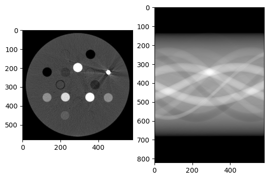
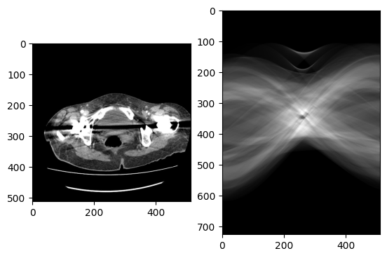
データはこのようになります。

# 論文から8 bit画像を画面キャプチャーでお借りました。
gammex 467 : https://ro-journal.biomedcentral.com/articles/10.1186/1748-717X-9-114#additional-information
# リンクからダウンロードしました。
adb : Case courtesy of Dinesh Brand, Radiopaedia.org, rID: 67631

これらを読み込みます。

gam_path = 'Gammex467.tif'
abd_path = 'ct-metal-artifact-reduction-single-energy-metal-artifact-reduction-semar-algorithm.jpg'
semar_path = 'ct-metal-artifact-reduction-single-energy-metal-artifact-reduction-semar-algorithm_SEMAR.jpg'

画像を読み込みます。

# 8 bit image (本当は16-bitで検討したいのですが、データがないので)
'''
gam = io.imread(gam_path) # numpy.ndarray
gam = img_as_float(gam)
abd = io.imread(abd_path)
abd = img_as_float(abd)
semar = io.imread(semar_path)
semar = img_as_float(semar)

正規化関数です。
今回は簡略化して、MinMaxスケールでいきます。

def normalize(image):
    im = image.copy()
    im = (im - np.min(im)) / (np.max(im) - np.min(im))
    return np.clip(im, 0.0, 1.0)

しきい値処理の関数です。
しきい値未満は0.0、以上はそのままにします。

def clip(image, threshold):
    im = image.copy()
    clipped = np.where(im<threshold, 0.0, im)
    return clipped

画像とサイノグラムを表示する関数です。

def show_image(image, sinogram):
    plt.subplot(1,2,1)
    plt.imshow(image, cmap='gray')
    plt.subplot(1,2,2)
    plt.imshow(sinogram, cmap='gray')
    plt.show()

サイノグラムの画素補間のための関数です。
(本当は、縦横だけでなく、斜めとかからも補間できるとよいのだろうか)

def interpolate_nan_columns(arr, kind='linear'):
    '''
    arr : adarray
    kind: linear, nearest, cubic
    '''
    for j in range(arr.shape[1]):
        y = arr[:, j]
        nans = np.isnan(y)
        if nans.all():
            continue  # 全ての値がNaNの場合、補間しない
        x = np.arange(len(y))
        f = interp1d(x[~nans], y[~nans], kind=kind, fill_value='extrapolate')
        arr[nans, j] = f(x[nans])
    return arr

def interpolate_nan_rows(arr, kind='linear'):
    for i in range(arr.shape[0]):
        y = arr[i, :]
        nans = np.isnan(y)
        if nans.all():
            continue  # 全ての値がNaNの場合、補間しない
        x = np.arange(len(y))
        f = interp1d(x[~nans], y[~nans], kind=kind, fill_value='extrapolate')
        arr[i, nans] = f(x[nans])
    return arr

画素補間でなく、欠損データの補間として扱うこともできます。
例えば、kNNやMICEなどですね。
ただ、今回はあまりうまく行かなかったので、紹介のみです。

def knn_impute(arr, nn=5):
    imputer = KNNImputer(n_neighbors=nn)
    return imputer.fit_transform(arr)

MARの関数です。
私の気分で書いていますので、アルゴリズムは、実際と違うところが含まれると思います。

def calc_mar(image, threshold, filter='ramp', interp='cubic'):
    '''
    filter
        ramp        高解像度が必要な場合
        shepp-Logan	バランス重視の再構成
        cosine      ノイズの多いデータ
        hamming	    ノイズと解像度のバランス
        hann	    非常にノイズの多いデータ
    interp
        ‘linear’, ‘nearest’, and ‘cubic’
    '''
    # preprocess
    # 正規化（MinMaxスケール）
    im_norm = normalize(image)
    # メタル画像の取得
    clipped = clip(im_norm, threshold)
    '''
    calc sinogram0 from org image
    '''
    # ラドン変換 180度の投影
    theta = np.linspace(0.0, 180.0, max(image.shape), endpoint=False)
    # org sinogram
    sinogram0 = radon(im_norm, theta=theta, circle=False)
    # metal sinogram
    sinogram1 = radon(clipped, theta=theta, circle=False)

    # original
    show_image(im_norm, sinogram0)
    print()
    # clip
    show_image(clipped, sinogram1)
    print()

    '''
    calculate no metal sinogram
    '''
    sinogram2 = sinogram0 - sinogram1
    # 改善の余地あり
    # 殆どがバックグラウンドな信号なので、簡易で中央値未満をNaNに。
    th = np.percentile(sinogram2, 50)
    # 0.0はバックグラウンド
    # 小さい値はアーチファクト領域など
    sinogram2[(sinogram2 > 0.0) & (sinogram2 < th)] = np.nan

    # interpolation
    sinogram2 = interpolate_nan_columns(sinogram2, kind=interp)
    sinogram2 = interpolate_nan_rows(sinogram2, kind=interp)

    # impute by knn
    # sinogram2 = knn_impute(sinogram2)

    # impute by imputer
    # imp_mean = IterativeImputer(max_iter=5, min_value=th, random_state=0)
    # imp_mean.fit(sinogram2)
    # sinogram2 = imp_mean.transform(sinogram2)

    '''
    reconstruct
    '''
    # filter : ramp, shepp-logan, cosine, hamming, hann
    # interpolation: ‘linear’, ‘nearest’, and ‘cubic’
    recon_nometal = iradon(sinogram2, theta=theta, filter_name=filter, interpolation='cubic', circle=False)

    # center crop (if you use circle=True, no need following cutout.)
    reconstructed_center = np.array(recon_nometal.shape) // 2
    original_center = np.array(image.shape) // 2
    start = reconstructed_center - original_center
    end = start + image.shape
    recon_nometal = recon_nometal[start[0]:end[0], start[1]:end[1]]

    # no metal
    show_image(recon_nometal, sinogram2)

    '''
    reduction
    '''
    sinogram3 = sinogram0 + sinogram2
    sinogram3 = normalize(sinogram3)
    recon_suppress = iradon(sinogram3, theta=theta, filter_name=filter, interpolation='cubic', circle=False)
    recon_suppress = recon_suppress[start[0]:end[0], start[1]:end[1]]
    recon_suppress = normalize(recon_suppress)

    show_image(recon_suppress, sinogram3)

    '''
    最後にメタル画像を加算
    '''
    mar_im = recon_suppress+(clipped)/2 # すべて加算すると強すぎるかもなので

    return mar_im

結果

gammex 467

res = calc_mar(gam, 0.9)
show_image(gam, res)

元画像

高信号領域のみの画像

差分画像

合成画像

MAR画像（左：ORG、右：処理結果）

あまり、アーチファクト消えていない（泣）

abd1

res1 = calc_mar(abd, 0.9)
show_image(gam, res1)

元画像

高信号領域のみの画像

差分画像

合成画像

MAR画像（左：ORG、右：処理結果）

サイノグラムの中心部の穴を補間でうまいことなくせたら、もっとうまくいくのだろう。

abd2(SEMAR済み)

元画像

高信号領域のみの画像

差分画像

合成画像

MAR画像（左：ORG、右：処理結果）

なんか、「おっ」ってなるけど、黒くなっただけ感あります。

References

• Ballhausen, H., Reiner, M., Ganswindt, U. et al. Post-processing sets of tilted CT volumes as a method for metal artifact reduction. Radiat Oncol 9, 114 (2014). https://doi.org/10.1186/1748-717X-9-114
• Brand D, CT metal artifact reduction - single energy metal artifact reduction (SEMAR) algorithm. Case study, Radiopaedia.org (Accessed on 26 Jun 2024) https://doi.org/10.53347/rID-67631
• Ichikawa K, Kawashima H, Takata T. An image-based metal artifact reduction technique utilizing forward projection in computed tomography. Radiol Phys Technol. 2024 Jun;17(2):402-411. doi: 10.1007/s12194-024-00790-1. Epub 2024 Mar 28. PMID: 38546970; PMCID: PMC11128408.

終わり

免責で書きましたが、ここでは、8-bit画像で試した結果のみを記録しました。本来、CTは16-bitで、かつ、HU値で操作できるので、16-bitでトライしたら、また違う結果になると思います。機会があればトライしたいです。

共同研究など、お声がけお待ちしております。

Stay visionary