環境
- Ubuntu 18.04
- Anaconda 1.9.6
- Tensorflow-gpu 1.12.0
- Keras-gpu 2.2.4
- GeForce GTX 1050 Ti(totalMemory: 3.95GiB freeMemory: 3.89GiB) + AkiTiONODE
※GPUを使いましたが、CPUでもできます。(確かめてませんが、、)
必要なもの
日本放射線技術学会「標準ディジタル画像データベース[胸部腫瘤陰影像]」Direction01
http://imgcom.jsrt.or.jp/minijsrtdb/
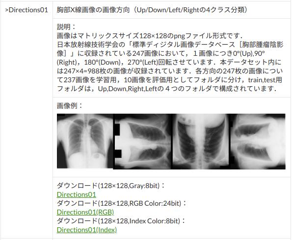
画像サイズ 128*128、色深度 Gray 8 bitのデータを選択してダウンロード。
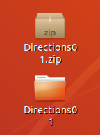
ダウンロードしたら解凍。ここではわかりやすくデスクトップへ。
Direction01.zipをデスクトップに移動して、右クリックから「ここで展開」を実行。
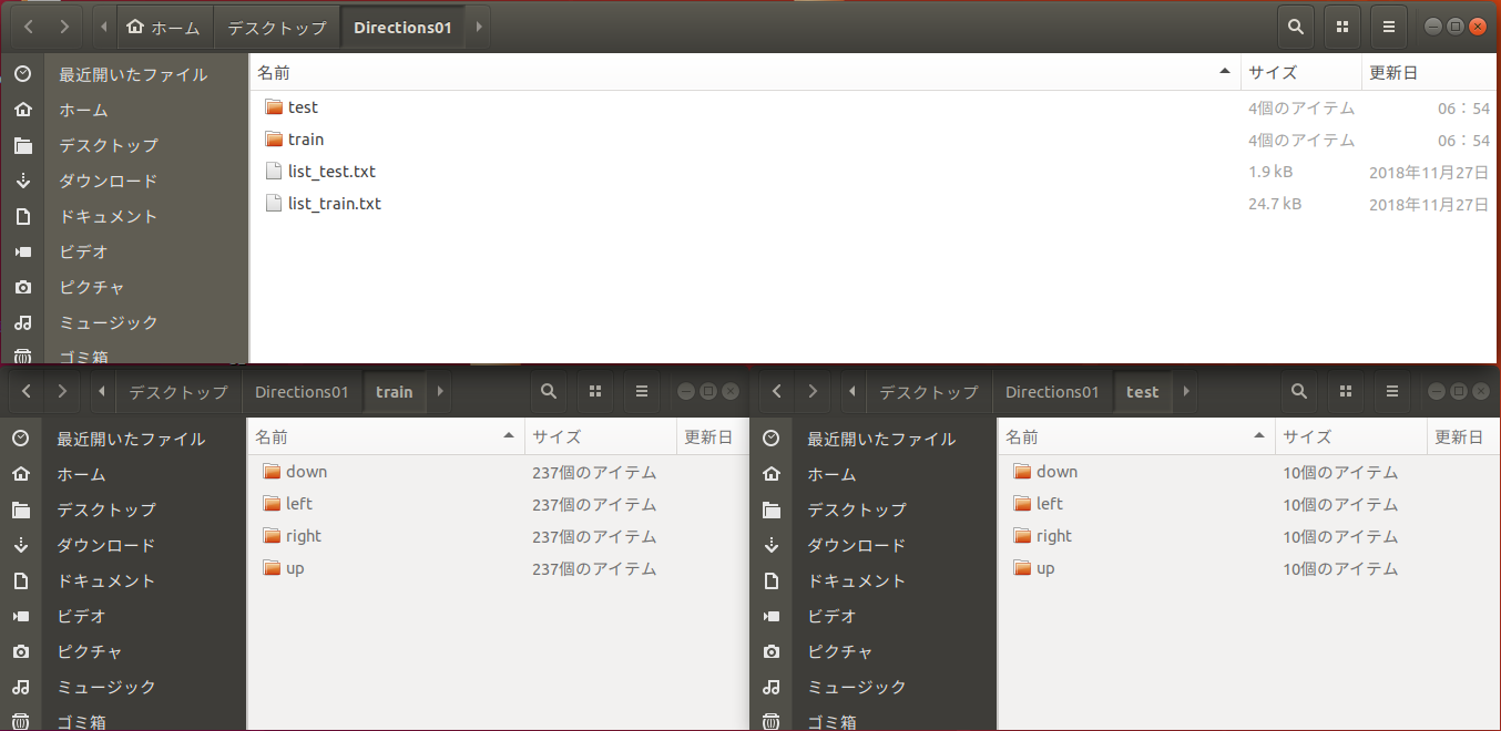
Direction01フォルダの中身は、とても親切に、トレーニングとテストデータが分かれており、かつ、それぞれのフォルダの中身も、Right, Left, down, upに整理されている。作成・提供者に感謝。
コード
さっそく、モデルをトレーニングしていく。
以下のような感じで試してみた。
'''
Created on 2019/05/03

@author: tatsunidas
'''

'''
必要なもの
Directions01のtrainとtestまでの絶対パス(フォルダの場所)
データジェネレータ(データを水増しする)
モデル(InceptionV3)
コールバック
トレーニング(categorical_crossentropy, Nadam, acc)
グラフ化
モデルとグラフの保存
テスト
'''

from keras.preprocessing.image import ImageDataGenerator
import keras
from keras.applications.inception_v3 import InceptionV3
from keras.layers import Dense, Flatten, BatchNormalization
from keras.models import Model
from keras.optimizers import Nadam
import matplotlib.pyplot as plt

# Directions01のtrainとtestまでの絶対パス(フォルダの場所)
'''
ここでは例を載せています。自分の環境に合わせて下さい。
例えば、Win10の方は、'C:\Users\あなたのユーザ名\Desktop'などになります。
'''
trainDir = '/home/tatsunidas/デスクトップ/Directions01/train'
testDir = '/home/tatsunidas/デスクトップ/Directions01/test'
# モデルの保存先と名前:ここでは例を載せています。自分の環境に合わせて下さい。
model_save_to = '/home/tatsunidas/デスクトップ/'
model_filename = 'model_best_directions01.h5'
plot_capture_to = '/home/tatsunidas/デスクトップ/result_plot.png'

# データのア(オ)ーギュメンテーション(水増し)の準備
datagen=ImageDataGenerator(
    rescale = 1./255,
    validation_split=0.2,#自動でバリデーションデータを分割させる
    rotation_range=20,
    width_shift_range=0.2,
    height_shift_range=0.2,
    shear_range=0.2,
    zoom_range=0.2,
    fill_mode='nearest',
    horizontal_flip=False,#今回はローテーション画像の判定なのでFalseのままにしておく
    vertical_flip=False#今回はローテーション画像の判定なのでFalseのままにしておく
    )
# 画像処理しながらトレーニングデータの水増しをしてくれるように設定
train_generator = datagen.flow_from_directory(
    trainDir,
    target_size=(299, 299),
    color_mode = "grayscale",
    class_mode='categorical',
    batch_size=10,
    shuffle=True,
    subset='training'
    )
# 画像処理しながらバリデーションデータを入力してくれるように設定
val_generator = datagen.flow_from_directory(
    trainDir,
    target_size=(299, 299),
    color_mode = "grayscale",
    class_mode='categorical',
    batch_size=10,
    shuffle=True,
    subset='validation'
    )

# callback
"""
トレーニング中に学習をさせているにも関わらず損失値が下がらなくなったら途中で終了させる設定。
ただし、単に中断するのではなく、何回か継続させてみて、それでも改善が見られない場合に中断するようにしている。
"""
callbacks_list = [
    #損失が一番小さいとき、モデルの重みを保存(あくまでも「重み」であることに注意)
    keras.callbacks.ModelCheckpoint(
        filepath=model_save_to+model_filename,
        monitor = 'val_loss',
        save_best_only=True
        ),
    # 損失が改善しなくなったら、継続して学習を10回チャンレンジさせる
    keras.callbacks.EarlyStopping(
        monitor='val_loss',
        patience=10#もっと小さくてよい
        ),
    # 損失が改善しなくなったら、7回目で学習率を0.1下げてみる
    keras.callbacks.ReduceLROnPlateau(
        monitor='val_loss',
        factor=0.1,
        patience=7#もっと小さくてよい
        ),
    # tensorboardという学習過程をブラウザで可視化するための設定。
#     keras.callbacks.TensorBoard(
#         log_dir=tflogDir,
#         histogram_freq=1,
#         embeddings_freq=1
#         )
    ]

# modelの構築
# インセプションV3をランダム初期化。特徴抽出部分に使う。
base_model_v3 = InceptionV3(include_top=False, weights=None ,input_shape=(299,299,1))
# 分類部分を追加
x = base_model_v3.output
x = Flatten()(x)
x = BatchNormalization()(x)
x = Dense(256, activation='relu')(x)
x = Dense(128, activation='relu')(x)
x = Dense(64, activation='relu')(x)
preds = Dense(4, activation='softmax')(x)# 今回は4クラスの分類なので
model = Model(inputs=base_model_v3.input, outputs=preds)
# モデルの構造を確認
model.summary()
# モデルを固定
# 多クラス分類・シングルラベルなので、loss="categorical_crossentropy",metrics=['accuracy']
model.compile(optimizer=Nadam(lr=2e-5),loss="categorical_crossentropy",metrics=['accuracy'])
# 計算量を分散するためにエポック内でステップを分割
STEP_SIZE_TRAIN=train_generator.samples//train_generator.batch_size
STEP_SIZE_VALID=val_generator.samples//val_generator.batch_size
# モデルのトレーニング
history = model.fit_generator(generator=train_generator,
                    steps_per_epoch=STEP_SIZE_TRAIN,
                    validation_data = val_generator,
                    validation_steps = STEP_SIZE_VALID,
                    callbacks=callbacks_list,
                    epochs=100#例えば最大100回学習の場合
                    )
# 最後のモデルの保存
model.save(filepath=model_save_to+'model_last.h5', overwrite=False, include_optimizer=True)

# トレーニング過程をグラフ化
fig, (axL, axR) = plt.subplots(ncols=2, figsize=(10,4))
# loss
def plot_history_loss(fit):
    # Plot the loss in the history
    axL.plot(fit.history['loss'],label="loss for training")
    axL.plot(fit.history['val_loss'],label="loss for validation")
    axL.set_title('model loss')
    axL.set_xlabel('epoch')
    axL.set_ylabel('loss')
    axL.legend(loc='upper right')
# acc
def plot_history_acc(fit):
    # Plot the loss in the history
    axR.plot(fit.history['acc'],label="acc for training")
    axR.plot(fit.history['val_acc'],label="acc for validation")
    axR.set_title('model accuracy')
    axR.set_xlabel('epoch')
    axR.set_ylabel('accuracy')
    axR.legend(loc='upper right')

plot_history_loss(history)
plot_history_acc(history)
fig.savefig(plot_capture_to)
plt.close()

'''
最後にテストデータをモデルに予測させて精度を確かめる
'''
test_datagen = ImageDataGenerator(
    rescale = 1./255
    )

test_generator = test_datagen.flow_from_directory(
    testDir,
    target_size=(299, 299),
    color_mode = "grayscale",
    class_mode='categorical',
    batch_size=5,
    shuffle=False
    )

STEP_SIZE_TEST=test_generator.samples//test_generator.batch_size

test_gen=model.predict_generator(
    test_generator,
    steps=STEP_SIZE_TEST,
    verbose=1
    )

# 精度を出力
print(model.evaluate_generator(generator=test_generator,
                               steps=STEP_SIZE_TEST,
                               verbose = 1))
結果
学習が終了すると、テストが自動で処理され、コンソールにテスト結果が出力される。
[0.0001470107831664791, 1.0]
左が損失値、右が精度。このデータセットに対しては、ほぼ完璧なモデルになった。
作成される成果物
コード内で指定した場所に以下のファイルが作成される。
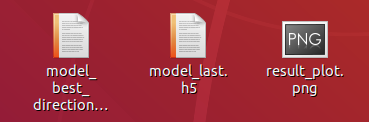
今回の学習の過程は、result_plot.pngを見れば確認できる。
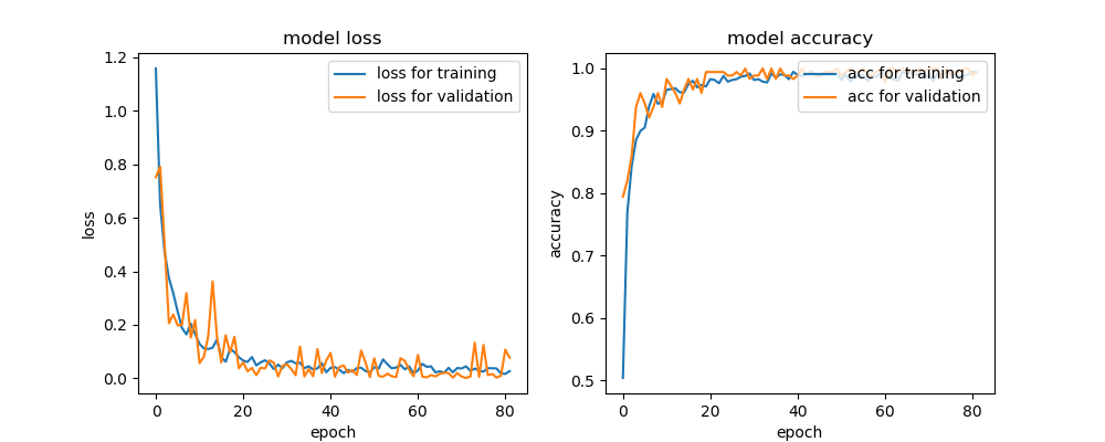
過学習をすれすれでコラえながら学習していることがわかる。
この記事を書いたモチベーション
備忘録として見返すと楽しそうと思ったから。
その他
コメント歓迎です。誤りなどもご指摘いただけましたら、時間のあるときに修正させていただきます。
参考URL
JSRT画像部会「MINIJSRT_DATABASE」:http://imgcom.jsrt.or.jp/minijsrtdb/
グラフ部分:https://qiita.com/hiroyuki827/items/213146d551a6e2227810