動機
備忘録として。
できること
画像を指定したクラス数にガウシアンフレームワークでセグメントする。
使ったもの
- NotebookLM
- 論文:Zhang Y, Brady M, Smith S. Segmentation of brain MR images through a hidden Markov random field model and the expectation-maximization algorithm. IEEE Trans Med Imaging. 2001 Jan;20(1):45-57. doi: 10.1109/42.906424. PMID: 11293691.
何がしたかったか
FSLのFASTで利用されているアルゴリズムを概念的に理解して、初歩的なコードに落とし込みたかった。
画像を統計的に扱う上で重要な数学的解釈や表現が詰まっているとても勉強になる論文だと思う。正直、マルコフランダム場、有限混合モデル、など、筆者にとってはあまり馴染みのない概念が論文の中で登場するので筆者には読み解くのがとても難しかった。例えば、解説されている数式が現実世界のどの変数に当てはまるのか、そして、自分で予想したそれは正しいのかどうかを確かめていく作業は、一連の知識を理解するためにトライアンドエラーを繰り返すことを必要とする。
しかし、NotebookLMのおかげで高等数学に弱い私でも概念的に理解できた。
概要
要は、ピクセル1つ1つを操作して、その近傍ピクセルがどのクラスに属しているかの割合を計算し、セグメンテーションラベルを更新していく。セグメンテーションする各クラスの平均と標準偏差を先に与えておくことで、各ピクセルがあるクラスに属する確率を求めるガウシアンアプローチができる。
概念的実装(NotebookLM利用+最終化は筆者)
import numpy as np
import random
import matplotlib.pyplot as plt

# 仮定する関数や変数:
# - y: 観測された画像データ (numpy array)
# - initial_labels: 初期ラベル配置 (numpy array, yと同じ形状)
# - K: クラスの数
# - mu: 各クラスの輝度平均 (リストや配列, サイズK)
# - sigma: 各クラスの輝度標準偏差 (リストや配列, サイズK)

def mrf_map_icm(y, initial_labels, K, mu, sigma, get_neighbors, max_iterations=100):
    """
    MRF-MAP推定のためのICMアルゴリズムの概念的実装
    """
    labels = initial_labels.copy()
    height, width = y.shape # 画像のサイズ (2Dを仮定)
    sites = [(i, j) for i in range(height) for j in range(width)] # 全サイトのリスト

    for iteration in range(max_iterations):
        print(f"Iteration {iteration+1}/{max_iterations}...")
        labels_changed_count = 0

        # サイトをランダムな順序で処理するとより良いことがあるが、ここでは簡単な順序で
        for s in sites:
            r, c = s # サイトの座標

            current_label = labels[r, c]
            min_energy = float('inf')
            best_label = current_label

            # 可能なすべてのクラスラベルを試す
            for k in range(K):
                # サイトsのラベルをkに仮定した場合の局所的な事後エネルギーを計算
                # 事後エネルギー = 事前エネルギー + 尤度エネルギー + const
                # ICMでは、サイトs以外のラベルは固定なので、
                # 変化するのはサイトsに関する尤度エネルギー項と、
                # サイトsを含む事前エネルギー項のみ

                # 尤度エネルギー項(式 17 のサイトsに関する項)
                # GHMRFでガウス分布を仮定 (式 15, 17)
                # E_L_s = (y_s - mu_{x_s})^2 / (2*sigma_{x_s}^2) + log(sqrt(2*pi)*sigma_{x_s})
                # 定数項 log(sqrt(2*pi)) はラベルkに依存しないので省略可能
                if sigma[k] == 0: # 分散がゼロの場合は無限大エネルギー (起こりえないラベル)
                     likelihood_energy_s = float('inf')
                else:
                     likelihood_energy_s = (y[r, c] - mu[k])**2 / (2 * sigma[k]**2) + np.log(sigma[k]) # np.log(np.sqrt(2*np.pi))は定数なので省略

                # 事前エネルギー項の変化分を計算
                # これはサイトsのラベルが現在のcurrent_labelからkに変わった際に
                # 事前エネルギーE(x)がどれだけ変化するかを表す。
                # 実際の計算は、MRFのポテンシャル関数E(x)の定義(式6など)に依存する。
                # 通常、隣接サイトのラベルとの関係に基づいて計算される。
                # ここでは概念的な関数呼び出しとする。
                # 例: 隣接サイトとのラベルが異なる場合にペナルティが加算される場合など
                neighbors_s = get_neighbors(s, height, width) # get_neighbors関数は実装による
                prior_energy_change = calculate_prior_energy_s_neighbors_pairwise(s, current_label, labels, neighbors_s)

                # サイトsのラベルをkとした場合の全体の事後エネルギーの変化または局所エネルギーを計算
                # ここでは、サイトsのラベルをkとした場合の局所的なエネルギーとして計算
                # 局所的事後エネルギーは、サイトsに関する尤度エネルギーと、サイトsを含むクリックの事前エネルギーの合計に比例
                # 簡易的には、サイトsの尤度エネルギー + サイトsと隣接サイトの事前エネルギー項の合計
                # ICM更新では、delta Energy を計算する方が効率的だが、概念的には局所エネルギーを評価する
                # 局所エネルギー = 尤度エネルギー(s) + 事前エネルギー(sと隣接サイト)
                # 事前エネルギー(sと隣接サイト) の計算は calculate_prior_energy_s_neighbors に任せる (実装詳細による)
                local_prior_energy = calculate_prior_energy_s_neighbors_pairwise(s, k, labels, neighbors_s) # サイトsのラベルをkとした場合の局所事前エネルギー計算 (概念)

                local_posterior_energy = likelihood_energy_s + local_prior_energy

                # 最小エネルギーとなるラベルを見つける
                if local_posterior_energy < min_energy:
                    min_energy = local_posterior_energy
                    best_label = k

            # 最適なラベルに更新
            if best_label != current_label:
                labels[r, c] = best_label
                labels_changed_count += 1

        # ラベルが全く変化しなければ収束
        if labels_changed_count == 0:
            print("ICM converged.")
            break

    return labels

# 隣接サイト取得関数 (例: 4近傍)
def get_neighbors_4(s, h, w):
    r, c = s
    neighbors = []
    for dr, dc in [(-1, 0), (1, 0), (0, -1), (0, 1)]:
        nr, nc = r + dr, c + dc
        if 0 <= nr < h and 0 <= nc < w:
            neighbors.append((nr, nc))
    return neighbors

# 局所事前エネルギー計算関数 (例: pairwise MRF, ラベルが一致するとエネルギーが低くなる)
def calculate_prior_energy_s_neighbors_pairwise(s, label_s, labels, neighbors_s, beta=1.0):
    energy = 0
    for nr, nc in neighbors_s:
        if label_s != labels[nr, nc]: # ラベルが一致しない場合にペナルティ
            energy += beta
    return energy

def generate_cow_like_pattern(width, height, brightness_val1, brightness_val2, brightness_val3):
    """
    指定された3つの輝度値を使用して、牛の模様風の画像を生成します。

    Args:
        width (int): 画像の幅 (ピクセル単位)。
        height (int): 画像の高さ (ピクセル単位)。
        brightness_val1 (int): 1つ目の輝度値 (0-255)。
        brightness_val2 (int): 2つ目の輝度値 (0-255)。
        brightness_val3 (int): 3つ目の輝度値 (0-255)。
        filename (str): 保存する画像ファイル名。
    """

    # 輝度値をソートして役割を割り当てます(背景、主たる斑点、副次的な斑点)。
    values = sorted([brightness_val1, brightness_val2, brightness_val3])
    bg_color = values[2]      # 最も明るい値を背景色とします (例: 220)
    spot_color_main = values[0] # 最も暗い値を主要な斑点の色とします (例: 25)
    spot_color_secondary = values[1] # 中間の値を副次的な斑点の色とします (例: 125)

    # 背景色で画像を初期化
    image_array = np.full((height, width), bg_color, dtype=np.uint8)

    # 複数の円を重ねて不規則な「ブロブ」(斑点)を描画する関数
    def draw_blob(arr, center_x, center_y, max_blob_radius, num_circles_per_blob, color_val):
        for _ in range(num_circles_per_blob):
            # ブロブを構成する個々の円の半径
            r = random.uniform(max_blob_radius * 0.3, max_blob_radius)

            # ブロブの中心から少しずらして、より不規則な形状を生成
            offset_x = random.uniform(-max_blob_radius * 0.5, max_blob_radius * 0.5)
            offset_y = random.uniform(-max_blob_radius * 0.5, max_blob_radius * 0.5)

            circ_center_x = center_x + offset_x
            circ_center_y = center_y + offset_y

            # 円のバウンディングボックスを取得してピクセル処理を効率化
            min_x = max(0, int(circ_center_x - r))
            max_x = min(width, int(circ_center_x + r) + 1)
            min_y = max(0, int(circ_center_y - r))
            max_y = min(height, int(circ_center_y + r) + 1)

            for y_coord in range(min_y, max_y):
                for x_coord in range(min_x, max_x):
                    # 円の内側のピクセルであれば色を塗る
                    if (x_coord - circ_center_x)**2 + (y_coord - circ_center_y)**2 < r**2:
                        arr[y_coord, x_coord] = color_val

    # 主要な斑点(暗い色)のパラメータと描画
    num_main_blobs = random.randint(4, 7) # 斑点の数
    for _ in range(num_main_blobs):
        blob_cx = random.randint(0, width - 1)  # 斑点の中心X座標
        blob_cy = random.randint(0, height - 1) # 斑点の中心Y座標
        # 斑点の最大半径 (画像の幅に対する相対値)
        blob_radius = random.uniform(width * 0.1, width * 0.25)
        circles_in_blob = random.randint(3, 7) # 1つの斑点を構成する円の数 (多いほど複雑)
        draw_blob(image_array, blob_cx, blob_cy, blob_radius, circles_in_blob, spot_color_main)

    # 副次的な斑点(中間色)のパラメータと描画
    num_secondary_blobs = random.randint(2, 4)
    for _ in range(num_secondary_blobs):
        blob_cx = random.randint(0, width - 1)
        blob_cy = random.randint(0, height - 1)
        blob_radius = random.uniform(width * 0.05, width * 0.15) # やや小さめの斑点
        circles_in_blob = random.randint(2, 5)
        draw_blob(image_array, blob_cx, blob_cy, blob_radius, circles_in_blob, spot_color_secondary)
    return image_array
テスト
# データとパラメータを準備 (例)
# 予測対象画像
y = generate_cow_like_pattern(100,100, 25,125,220)

print("y")
plt.imshow(y)
plt.show()

K = 3 # 3クラス
initial_labels = np.random.randint(0, K, size=y.shape) # ランダムな初期ラベル

mu = [25, 125, 220] # 各クラスの平均輝度
sigma = [0.3, 0.3, 0.3] # 各クラスの標準偏差

# ICMを実行
estimated_labels = mrf_map_icm(y, initial_labels, K, mu, sigma, get_neighbors_4, max_iterations=10)

# 結果として estimated_labels に推定されたラベル配置が得られる
print("estimate result")
plt.imshow(estimated_labels)
plt.show()
y画像

セグメンテーション結果

MRI画像(T1w)でテスト
import requests
import zipfile
import io
import numpy as np
import tifffile # TIFFファイルの読み込みに特化したライブラリ

def download_and_extract_tiff_zip_to_ndarray(url: str) -> np.ndarray | None:
    """
    指定されたURLからZIPファイルをダウンロードし、その中のTIFFファイルを読み込んで
    NumPy配列として返します。
    ZIPファイルには単一のマルチページTIFF、または複数のシングルページTIFFが含まれていることを想定しています。

    Args:
        url (str): TIFFファイルを含むZIPファイルのURL。

    Returns:
        np.ndarray | None: 成功した場合は画像データを含むNumPy配列、失敗した場合はNone。
    """
    try:
        # 1. ZIPファイルをダウンロード
        print(f"'{url}' からZIPファイルをダウンロードしています...")
        response = requests.get(url, timeout=30)
        response.raise_for_status()  # HTTPエラーがあれば例外を発生させる
        zip_file_bytes = io.BytesIO(response.content)
        print("ダウンロード完了。")

        tiff_image_data = None

        with zipfile.ZipFile(zip_file_bytes) as zf:
            # ZIPファイル内のTIFFファイル名を取得 (.tif または .tiff)
            tiff_file_names = [name for name in zf.namelist() if name.lower().endswith(('.tif', '.tiff'))]

            if not tiff_file_names:
                print("エラー: ZIPファイル内にTIFFファイルが見つかりませんでした。")
                return None

            print(f"ZIP内で見つかったTIFFファイル: {tiff_file_names}")

            # ケース1: ZIP内に単一のTIFFファイルが存在する場合 (多くはマルチページTIFFスタック)
            if len(tiff_file_names) == 1:
                file_name = tiff_file_names[0]
                print(f"単一のTIFFファイル '{file_name}' を処理しています...")
                with zf.open(file_name) as specific_file_bytes:
                    # tifffile.imread はファイルライクオブジェクトから直接読み込める
                    tiff_image_data = tifffile.imread(specific_file_bytes)
                print(f"'{file_name}' の読み込み成功。形状: {tiff_image_data.shape}, データ型: {tiff_image_data.dtype}")

            # ケース2: ZIP内に複数のTIFFファイルが存在する場合 (各ファイルがスライスであると仮定)
            else:
                print(f"複数のTIFFファイルが見つかりました。これらをスライスとして結合します: {tiff_file_names}")
                # ファイル名でソートして、スライスの順序を正しく保つ (例: slice01.tif, slice02.tif ...)
                tiff_file_names.sort()

                slices = []
                for file_name in tiff_file_names:
                    print(f"スライス '{file_name}' を読み込んでいます...")
                    with zf.open(file_name) as specific_file_bytes:
                        slice_data = tifffile.imread(specific_file_bytes)
                        slices.append(slice_data)

                if not slices:
                    print("エラー: TIFFスライスからデータを読み込めませんでした。")
                    return None

                try:
                    # スライスをNumPy配列としてスタック (通常、スライス方向が最初の次元になるように)
                    tiff_image_data = np.stack(slices, axis=0)
                    print(f"全{len(slices)}スライスのスタック成功。最終的な形状: {tiff_image_data.shape}, データ型: {tiff_image_data.dtype}")
                except ValueError as e:
                    print(f"エラー: スライスのスタックに失敗しました。各スライスの形状が異なる可能性があります。詳細: {e}")
                    return None

        return tiff_image_data

    except requests.exceptions.RequestException as e:
        print(f"ダウンロードエラー: {e}")
        return None
    except zipfile.BadZipFile:
        print("エラー: ZIPファイルが壊れているか、不正な形式です。")
        return None
    except tifffile.TiffFileError as e: # tifffile固有のエラー
        print(f"TIFファイルの読み込みエラー: {e}")
        return None
    except Exception as e:
        print(f"予期せぬエラーが発生しました: {e}")
        return None
実行
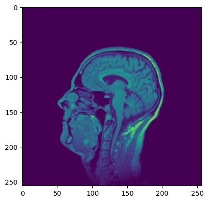
t1 = download_and_extract_tiff_zip_to_ndarray("https://imagej.net/ij/images/t1-head.zip")
plt.imshow(t1[63, :,:])
plt.show()
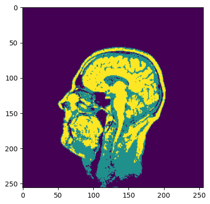
K = 3 # 3クラス(白質、灰白質、脳脊髄液)
initial_labels = np.random.randint(0, K, size=(256,256)) # ランダムな初期ラベル
mu = [180, 340, 50] # 各クラスの平均輝度
sigma = [20, 7, 12] # 各クラスの標準偏差
# ICMを実行
estimated_labels = mrf_map_icm(t1[63, :,:], initial_labels, K, mu, sigma, get_neighbors_4, max_iterations=100)
# 結果として estimated_labels に推定されたラベル配置が得られる
print("estimate result")
plt.imshow(estimated_labels)
plt.show()

今回は背景(空気や頭蓋骨など脳以外の領域)を含めているが、実際は頭蓋骨除去を行ってから処理するので、背景情報は無視できる。
平均値と標準偏差を適切に指定したり、処理前にデノイズしておいたりすることで、より精度を高めることができる。
バイアスフィールド補正を考慮する
先の例では、シンプルにSiteのピクセルがどのクラスに属しそうかを近傍ピクセルの個数から推定するアプローチだった。
しかし、このアプローチの課題はノイズに弱いことである。
例えば、MRI画像などは画像信号にノイズを含むため、そのノイズの量を考慮してクラスラベルが推定されるべきである。
これをコードに落とし込んでみる。
処理の流れは以下の通り。
- まず、初期パラメータ(平均値と標準偏差)を推定する
- 予測ラベルと事後確率マップをMRFマップから取得する
- 事後確率マップを使ってバイアスフィールドを推定する
- 収束するまで繰り返す
import numpy as np
import matplotlib.pyplot as plt
from skimage.filters import threshold_multiotsu
# scikit-imageライブラリを使用する場合の例
# インストールが必要: pip install scikit-image
def initialize_parameters_from_histogram(data, num_classes):
    # データは0-255の範囲にクリップすることが多い
    # data = np.clip(data, 0, 255).astype(np.uint8)

    # 2. データのヒストグラムを計算
    #    ソース [1] で初期推定にヒストグラム分析が用いられると述べられている
    hist, bins = np.histogram(data.ravel(), bins=256, range=(data.min(), data.max()))
    bin_centers = (bins[:-1] + bins[1:]) / 2

    # 3. 多クラスOtsu法を適用して閾値を計算 (3クラス分類の場合、閾値は2つ得られる)
    #    ソース [1] で「クラス間分散を最大化する閾値を見つける」と述べられている処理に該当
    thresholds = threshold_multiotsu(data, classes=num_classes)
    print(f"計算された閾値 (skimage): {thresholds}")

    # 4. 計算された閾値を使用してデータを3つのクラスに分類
    #    ソース [1] で「初期分類も、この閾値処理によって直接...得られる」と述べられている処理に該当
    #    閾値 t1, t2 (t1 < t2) に対して、クラス1: < t1, クラス2: t1 <= < t2, クラス3: >= t2
    class_labels = np.zeros_like(data, dtype=int)
    mu = []
    sigma = []
    k = 0
    for th in thresholds:
        class_labels[data >= th] = k+1
        k += 1

    for k in range(num_classes):
        m = np.mean(data[class_labels == k])
        sd = np.std(data[class_labels == k])
        mu.append(m)
        sigma.append(sd)

    print("\n最終的な初期パラメータ:")
    print(f"初期平均: {mu}")
    print(f"初期標準偏差: {sigma}")

    # # オプション:ヒストグラムと閾値、クラス分けの様子を可視化
    # plt.figure(figsize=(7, 4))
    # plt.hist(data, bins=256, range=(data.min(), data.max()), density=False, alpha=0.6, label='Histogram')
    # for t in thresholds:
    #     plt.axvline(t, color='r', linestyle='dashed', linewidth=2, label=f'Threshold = {t:.2f}')

    # # 分類されたクラスの平均をプロット(概念として)
    # colors = ['b', 'g', 'm']
    # class_means_by_label = [np.mean(data[class_labels == i]) for i in range(3) if np.sum(class_labels == i) > 0]
    # for i, mean_val in enumerate(class_means_by_label):
    #     plt.axvline(mean_val, color=colors[i], linestyle='dotted', linewidth=2, label=f'Class {i} Mean')

    # plt.title('Histogram with Otsu Thresholds and Initial Means (Conceptual)')
    # plt.xlabel('Intensity Value')
    # plt.ylabel('Frequency (Normalized)')
    # plt.yscale('log')
    # plt.legend()
    # plt.grid(True)
    # plt.show()
    return class_labels, mu, sigma
import numpy as np
import math
from scipy.special import softmax

def calculate_prior_energy(current_label, neighbors_labels, beta):
    """
    # MRF priorのエネルギー関数 (Potts model)
    # エネルギーが低いほど確率が高い -> Pは exp(-Energy) に比例
    # ここでは条件付き確率 P(x_s | x_N_s) を計算するために、
    # ラベルkに対するエネルギー U_prior(x_s=k | x_N_s) を定義
    Calculate the prior energy for a given label at a pixel based on its neighbors' labels.
    Using a simple Potts model: penalize differences with neighbors.
    U_prior(x_s | x_N_s) = beta * sum_{t in N_s} I(x_s != x_t)
    Lower energy means higher prior probability.
    """
    energy = 0
    for neighbor_label in neighbors_labels:
        if current_label != neighbor_label:
            energy += beta
    return energy

# Gaussian尤度関数 (対数スケール)
# バイアス場 b_s を考慮した Gaussian N(y_s | b_s*mu_k, (b_s*sigma_k)^2)
# 対数尤度: log P(y_s | x_s=k, b_s, mu_k, sigma_k)
# = -log(b_s * sigma_k) - (y_s - b_s*mu_k)^2 / (2 * (b_s*sigma_k)^2) - 0.5*log(2*pi)
# const項は無視できるため、前半2項を計算
def calculate_log_likelihood(observed_intensity, class_mu, class_sigma, bias_field_value):
    """
    Calculate the log-likelihood for an observed intensity given a class and bias field.
    Based on N(y_s | b_s * mu_k, (b_s * sigma_k)^2).
    Assumes mu_k and sigma_k are for the ideal intensity distribution.
    """
    # Handle potential zero sigma_k or bias_field_value for numerical stability
    effective_sigma = bias_field_value * class_sigma
    if effective_sigma < 1e-7: # Prevent division by zero or very small numbers
         effective_sigma = 1e-7

    # Calculate log-likelihood (ignoring constant term -0.5*log(2*pi))
    diff = observed_intensity - bias_field_value * class_mu
    # (diff ** 2) / (2 * effective_sigma ** 2) means these exponentials.
    log_lik = -np.log(effective_sigma) - (diff ** 2) / (2 * effective_sigma ** 2)

    return log_lik

# ICMアルゴリズムによるMRF-MAP推定
def estimate_labels_mrf_map(image_data,
                            initial_labels,
                            mu,
                            sigma,
                            bias_field,
                            beta,
                            num_classes,
                            neighborhood_system,
                            num_iterations):
    """
    Estimates class labels using the MRF-MAP criterion with the ICM algorithm.

    Args:
        image_data (np.ndarray): The original observed image data (not log-transformed).
        initial_labels (np.ndarray): Initial label assignment for each voxel.
        mu (np.ndarray): Array of mean values for each class (for ideal intensity). Shape (num_classes,).
        sigma (np.ndarray): Array of standard deviation values for each class (for ideal intensity). Shape (num_classes,).
        bias_field (np.ndarray): Estimated bias field. Same shape as image_data.
        beta (float): Parameter for the MRF prior. Controls smoothness.
        num_classes (int): Number of tissue classes.
        neighborhood_system: get_neighbors function (e.g. get_neighbors_4)
        num_iterations (int): Number of ICM iterations.

    Returns:
        np.ndarray: Updated label assignment for each voxel.
    """
    current_labels = np.copy(initial_labels)
    shape = image_data.shape
    height, width = shape # 画像のサイズ (2Dを仮定)
    sites = [(i, j) for i in range(height) for j in range(width)] # 全サイトのリスト
    posterior_probabilities = np.zeros((height, width, num_classes))

    for iter in range(num_iterations):
        print(f"ICM Iteration {iter + 1}/{num_iterations}")
        # Iterate through each voxel (simplified raster scan order)
        labels_changed_count = 0
        for s in sites:
            r, c = s # サイトの座標
            observed_intensity = image_data[s]
            current_label = current_labels[s]
            current_bias_value = bias_field[s]
            log_posterior_per_class = np.zeros(num_classes)
            neighbors_s = neighborhood_system(s, height, width) # get_neighbors関数は実装による
            # Get neighbors' labels
            neighbors_labels = []
            for j, i in neighbors_s:
                # Check boundary conditions
                if 0 <= j < width and 0 <= i < height:
                    neighbors_labels.append(current_labels[i,j])

            # For each possible class label (k) for the current voxel:
            for k in range(num_classes):
                # Calculate log-likelihood P(y_s | x_s=k, ...)
                # Use original intensity, bias field, and class params (mu, sigma)
                log_lik = calculate_log_likelihood(observed_intensity, mu[k], sigma[k], current_bias_value)

                # Calculate prior energy U_prior(x_s=k | x_N_s)
                prior_energy = calculate_prior_energy(k, neighbors_labels, beta)

                # Calculate log-posterior (up to a constant): log P(x_s | y_s, x_N_s) propto log P(y_s | ...) + log P(x_s | x_N_s)
                # Note: Maximizing log P(x_s | y_s, x_N_s) is equivalent to minimizing -log P(x_s | y_s, x_N_s).
                # log P(x_s | x_N_s) propto -U_prior(x_s | x_N_s)
                # So, log-posterior propto log_lik - prior_energy + const
                log_posterior_per_class[k] = log_lik - prior_energy

            # Select the label that maximizes the log-posterior (MAP estimate for this pixel)
            new_label = np.argmax(log_posterior_per_class)
            # posterior_probabilities[s[0], s[1],:] = np.exp(log_posterior_per_class)
            posterior_probabilities[s[0], s[1],:] = softmax(log_posterior_per_class)
            current_labels[r, c] = new_label
            if new_label != current_label:
                labels_changed_count += 1

        # ラベルが全く変化しなければ収束
        if labels_changed_count == 0:
            print("ICM converged.")
            break

    return current_labels, posterior_probabilities
from scipy.ndimage import gaussian_filter

def estimate_bias_field_map_conceptual(
    observed_image,          # 観測されたMR画像 (x_i)
    current_bias_field,      # 現在のバイアスフィールド推定値 (f_i)
    class_mus,               # 各クラスの平均強度 (mu_k)
    class_sigmas,            # 各クラスの標準偏差 (sigma_k)
    posterior_probabilities, # Eステップで計算された各ピクセルのクラス事後確率 P(z_i=k | x_i, f_i_current)
    gaussian_class_indices,  # 正規分布を仮定するクラスのインデックスリスト (Guillemaud & Brady [3] の修正用) [13, 14]
    bias_field_prior_params  # バイアスフィールドの事前分布に関するパラメータ(例: {'sigma_f_constant': 1.0} (ソース [7] の sigma_f に関連)
):
    """
    与えられた観測画像、現在のバイアスフィールド、クラスパラメータ、
    およびクラス事後確率に基づいて、MAP基準でバイアスフィールドマップを更新する (概念)。

    Args:
        observed_image (np.ndarray): 観測強度マップ。
        current_bias_field (np.ndarray): 現在のバイアスフィールド推定値マップ。
        class_mus (list or np.ndarray): 各クラスの平均強度のリストまたは配列。
        class_sigmas (list or np.ndarray): 各クラスの標準偏差のリストまたは配列。
        posterior_probabilities (np.ndarray): 各ピクセル、各クラスの事後確率マップ。
                                             形状: (画像高さ, 画像幅, [画像深さ], クラス数)。
        gaussian_class_indices (list): バイアスフィールド推定に使用する正規分布クラスのインデックス。
        bias_field_prior_params (dict): バイアスフィールド事前分布のパラメータ。
                                        例: {'sigma_f_constant': 1.0} (ソース [7] の sigma_f に関連)

    Returns:
        np.ndarray: 更新されたバイアスフィールドマップ。
    """
    image_dims = observed_image.shape

    # --- ステップ 1: Guillemaud and Brady の修正平均残差 (mu_epsilon_i) を計算 ---
    # ソース [13] 式(38) に基づき、正規分布を仮定するクラスのみを用いて計算。
    mu_epsilon_gb_map = np.zeros(image_dims)
    for k in gaussian_class_indices:
        mu_k = class_mus[k]
        # 画像全体でベクトル化された計算 (NumPyを利用)
        p_k_map = posterior_probabilities[..., k] # ...は全ての空間次元を指す
        # 平均残差の計算: p(z_i=k|...) * (x_i - mu_k * f_i) [45, 式(38)]
        mu_epsilon_gb_map += p_k_map * (observed_image - mu_k * current_bias_field)
    print("平均残差", mu_epsilon_gb_map.max(), mu_epsilon_gb_map.min())

    # --- ステップ 2: 平均逆共分散 (v_epsilon_i に関連する項) を計算 ---
    # ソース [7] 式(36) v_epsilon_i_inv = sum_k p(z_i=k|...) / (sigma_k*f_i)^2 に対応すると考えられます。
    v_epsilon_inv_map = np.zeros(image_dims)
    # 分散ゼロやバイアスフィールドゼロによる除算を防ぐための小さな値を設定
    min_effective_variance = 1e-9
    v_epsilon_inv_map += min_effective_variance
    for k in gaussian_class_indices:
        sigma_k = class_sigmas[k]
        p_k_map = posterior_probabilities[..., k]
        # 有効分散 (sigma_k * f_i)^2 [7]
        effective_variance_map = (sigma_k * current_bias_field) ** 2
        effective_variance_map += min_effective_variance
        # 有効な分散を持つピクセルのみ計算
        mask = effective_variance_map > min_effective_variance
        v_epsilon_inv_map[mask] += p_k_map[mask] / effective_variance_map[mask]
        # v_epsilon_inv_map += p_k_map / effective_variance_map
    print("逆共分散", v_epsilon_inv_map.max(), v_epsilon_inv_map.min())

    # --- ステップ 3: 空間フィルタリングの入力となる項を計算 ---
    # ソース [7] 式(33)の構造 f = K * [ K_input_term ] に従います。
    # 式(33)は f_i = [K * (f_i/v_epsilon_i)]_i * mu_epsilon_i - [K * (f_i^2 * sigma_f / v_epsilon_i)]_i
    # の形に整理できることが示唆されています。
    # ここで v_epsilon_i は v_epsilon_inv_i の逆数 1/v_epsilon_inv_i に対応します。
    # (ただし、この正確な関係はソース [9] に依存する可能性があります)

    # 計算を安定させるための小さな値を設定
    min_v_epsilon_inv = 1e-9
    valid_mask = v_epsilon_inv_map > min_v_epsilon_inv
    print("valid mask", valid_mask.sum())

    # v_epsilon_i を計算 (有効なピクセルのみ)
    v_epsilon_map = np.zeros(image_dims)
    v_epsilon_map[valid_mask] = 1.0 / v_epsilon_inv_map[valid_mask]
    # v_epsilon_map = 1.0 / v_epsilon_inv_map

    # フィルタリングされる第一項の入力マップ: f_i / v_epsilon_i [42, 式(33)内]
    f_over_v_map = np.zeros(image_dims)
    f_over_v_map[valid_mask] = current_bias_field[valid_mask] / v_epsilon_map[valid_mask]
    # f_over_v_map = current_bias_field / v_epsilon_map

    # フィルタリングされる第二項の入力マップ: f_i^2 * sigma_f / v_epsilon_i [42, 式(33)内]
    # sigma_f はバイアスフィールドの事前分布に関わるパラメータ [8]。
    # ソース [1] だけでは sigma_f のexact form は不明確ですが、式(33)に現れる形に基づき概念化します。
    # 例として、bias_field_prior_params から sigma_f に相当する定数 'sigma_f_constant' を取得します。
    sigma_f_constant = bias_field_prior_params.get('sigma_f_constant', 1.0)
    f_sq_sigma_f_over_v_map = np.zeros(image_dims)
    f_sq_sigma_f_over_v_map[valid_mask] = (current_bias_field[valid_mask]**2 * sigma_f_constant) / v_epsilon_map[valid_mask]
    # f_sq_sigma_f_over_v_map = (current_bias_field**2 * sigma_f_constant) / v_epsilon_map


    # --- ステップ 4: 空間フィルタ K を各入力マップに適用 ---
    '''
    sigmaは定数で調整
    '''
    filtered_f_over_v = apply_spatial_filter_conceptual(f_over_v_map, np.mean(sigma))
    filtered_f_sq_sigma_f_over_v = apply_spatial_filter_conceptual(f_sq_sigma_f_over_v_map, np.mean(sigma))


    # --- ステップ 5: フィルタリング結果と平均残差を組み合わせて新しいバイアスフィールドを計算 ---
    # ソース [7] 式(33)の構造 f_i = [K * (f_i/v_epsilon_i)]_i * mu_epsilon_i - [K * (f_i^2 * sigma_f / v_epsilon_i)]_i に従います。
    # ここで、[K * G]_i はフィルタ K をマップ G に適用した結果のピクセル i の値であり、
    # filtered_f_over_v および filtered_f_sq_sigma_f_over_v はこの結果マップです。
    # mu_epsilon_gb_map は各ピクセル i で既に計算されています (ステップ 1)。

    new_bias_field = filtered_f_over_v * mu_epsilon_gb_map - filtered_f_sq_sigma_f_over_v

    # new_bias_field = f_over_v_map * mu_epsilon_gb_map - f_sq_sigma_f_over_v_map

    # 注意: ソース [7] では、式 (33) がゼロ勾配条件から導かれるとされており、
    # これはバイアスフィールドを推定するための反復的な解法(例: Gauss-Seidel法など)の一部である可能性が高いです。
    # ここで計算される new_bias_field は、その反復における1ステップの結果、
    # または全体のEM反復におけるバイアスフィールドの新しい推定値として扱われます。

    # バイアスフィールドのクリッピング (非常に重要!)
    min_bias_value = 1e-2 # Or some other sensible lower bound
    new_bias_field = np.maximum(new_bias_field, min_bias_value)

    return new_bias_field

# ヘルパー関数 (概念的 - 実際の画像処理ライブラリ関数に置き換えられます)
def apply_spatial_filter_conceptual(image_map, sigma_k):
    return gaussian_filter(image_map, sigma=sigma_k)
# HMRF-EMによる脳MR画像セグメンテーションとバイアスフィールド補正の主関数
def segment_brain_mr_image_hmrf_em_bias_corrected(image_data, num_classes, max_iterations=100):
    """
    Args:
        image_data (numpy.ndarray): 入力となる3次元脳MR画像データ。
        num_classes (int): セグメンテーションする組織クラスの数(例: GM, WM, CSFのための3)。
                           非ガウス分布に対応する「その他」のクラスを含む場合もある。
        max_iterations (int): EMアルゴリズムの最大反復回数。

    Returns:
        tuple: (segmented_labels, estimated_bias_field, restored_image, estimated_parameters)
               概念的には、セグメンテーション結果、推定されたバイアスフィールド、
               バイアスフィールド補正済み画像、推定されたモデルパラメータを返します。
    """

    # 1. 初期化ステップ
    # EMアルゴリズムとラベル推定(ICMなど)は局所解に収束するため、初期条件が重要です。
    # 初期パラメータ(各クラスの平均、分散)および初期分類を推定します。
    # バイアスフィールドは初期にはゼロと仮定されることが多いです。
    print("Initializing HMRF-EM framework...")
    # ヒストグラム解析や閾値処理(例: 大津法)を用いて初期パラメータを推定することを想定。
    current_labels, mu, sigma = initialize_parameters_from_histogram(image_data, num_classes)
    # 初期バイアスフィールドは1と仮定。(これは対数変換バイアスフィールド初期値0に相当)
    estimated_bias_field = np.ones_like(image_data)
    posterior_probabilities = np.zeros([image_data.shape[0], image_data.shape[1], num_classes])
    best_labels = np.zeros_like(image_data)
    best_bias_field = np.zeros_like(image_data)
    best_posterior_probabilities = np.zeros_like(posterior_probabilities)
    best_score = 0.0
    no_updation = 0
    beta = 1/4 # from get_neighbors_4
    print("Initialization complete. Starting EM iterations...")

    # 2. EMアルゴリズムの反復
    # EステップとMステップを交互に繰り返すことで、パラメータと潜在変数(ここではラベルとバイアスフィールド)を推定します。
    for iteration in range(max_iterations):
        print(f"EM Iteration {iteration + 1}/{max_iterations}")

        # --- E-Step: 期待値の計算(ここでは、ラベルとバイアスフィールドの推定に相当) ---
        # このステップでは、現在のパラメータとバイアスフィールドの推定値を用いて、
        # データが与えられた下での隠れた変数(クラスラベルとバイアスフィールド)の確率や期待値を計算します。

        # 2a. クラスラベルの推定(MRF-MAP分類)
        # HMRFモデルの重要な点であり、隣接ピクセルの空間的な相互作用を考慮します。
        # 現在のパラメータとバイアスフィールド推定値を基に、各ピクセルのクラスラベルを推定します。
        # MRF-MAP推定は、事後確率を最大化することに相当し、エネルギー関数の最小化として定式化されます。
        # 最小化には、ICMなどの反復的局所最適化手法が用いられます。
        # ここで、MRFの事前分布(空間的な平滑性)がラベル推定に影響を与えます。
        new_labels, posterior_probabilities = estimate_labels_mrf_map(image_data,
                                                                      current_labels,
                                                                      mu,
                                                                      sigma,
                                                                      estimated_bias_field,
                                                                      beta,
                                                                      num_classes,
                                                                      get_neighbors_4,
                                                                      10)

        print("posterior probabilities at", iteration, posterior_probabilities.max(), posterior_probabilities.min())

        # 2b. バイアスフィールドの推定(MAP推定)
        # 現在のクラスラベル推定値と画像データを用いて、バイアスフィールドを推定します。
        # これはMAP原理に基づいて行われます。
        # 資料では、非ガウス分布クラスを「その他」として扱う修正EM(MEM)アプローチが統合されています。
        # 推定には、クラスごとの平均残差や逆共分散の計算、および低域通過フィルタリングが含まれます。
        estimated_bias_field = estimate_bias_field_map_conceptual(image_data,          # 観測されたMR画像 (x_i)
                                                                  estimated_bias_field,      # 現在のバイアスフィールド推定値 (f_i)
                                                                  mu,               # 各クラスの平均強度 (mu_k)
                                                                  sigma,            # 各クラスの標準偏差 (sigma_k)
                                                                  posterior_probabilities, # Eステップで計算された各ピクセルのクラス事後確率 P(z_i=k | x_i, f_i_current)
                                                                  range(num_classes),
                                                                  {'sigma_f_constant': 1.0}
                                                                  )

        print("current bias field", estimated_bias_field.max(), estimated_bias_field.min(), np.mean(estimated_bias_field))

        if posterior_probabilities.sum() > best_score:
            best_score = posterior_probabilities.sum()
            best_labels = np.copy(new_labels)
            best_bias_field = np.copy(estimated_bias_field)
            best_posterior_probabilities = np.copy(posterior_probabilities)
        else:
            no_updation += 1

        # 収束判定
        # パラメータの変化量や、クラスラベルの変化ピクセル数などが閾値以下になったら収束とみなします。
        if no_updation > 3:
            print(f"HMRF-EM converged at iteration {iteration + 1}")
            break

        # 次の反復のためにパラメータとラベルを更新
        for i in range(num_classes):
            mu[i] = np.mean(image_data[new_labels==i])
            sigma[i] = np.std(image_data[new_labels==i])
        current_labels = new_labels
        print("updated mu:", mu[0],mu[1],mu[2])
        print("updated sigma:", sigma[0],sigma[1],sigma[2])

        # # (バイアスフィールド補正を考慮したクラスパラメータの更新)
        # # 今回は、うまく収束しなかったので、オリジナル画像のみを利用
        # for k_class in range(num_classes):
        #     # クラス k_class に属するピクセルのインデックスを取得
        #     class_pixels_mask = (new_labels == k_class)
        #     if np.sum(class_pixels_mask) > 0: # クラスにピクセルが割り当てられている場合のみ更新
        #         # バイアス補正された強度を取得
        #         # estimated_bias_field がゼロや非常に小さい値を取らないように注意が必要
        #         # (前のステップでクリッピングされているはず)
        #         corrected_intensities = image_data[class_pixels_mask] / estimated_bias_field[class_pixels_mask]
        #         mu[k_class] = np.mean(corrected_intensities)
        #         sigma[k_class] = np.std(corrected_intensities)
        #         # sigma がゼロや非常に小さくならないように下限値を設けることも検討
        #         if sigma[k_class] < 1e-6: # 例: 非常に小さい標準偏差を防ぐ
        #             sigma[k_class] = 1e-6
        #     # else:
        #         # クラスにピクセルが割り当てられなかった場合の処理 (例: パラメータを維持、または再初期化の検討)
        #         # print(f"Warning: Class {k_class} has no pixels assigned in iteration {iteration + 1}. Parameters not updated.")
        # current_labels = new_labels
        # print("updated mu (bias corrected):", mu) # mu全体を表示する方が見やすいかも
        # print("updated sigma (bias corrected):", sigma) # 同上

    print("EM iterations finished.")

    # 3. 最終出力の準備
    # 最終的なセグメンテーション結果、推定バイアスフィールド、復元画像、推定パラメータを返します。
    return best_labels, best_bias_field, best_posterior_probabilities
実行
num_classes = 3
best_labels, best_bias_field, best_posterior_probabilities = segment_brain_mr_image_hmrf_em_bias_corrected(t1[63,:,:],
                                                                                                           num_classes,
                                                                                                           max_iterations=100)
plt.imshow(best_labels)
plt.imshow(best_bias_field)

for i in range(num_classes):
    plt.imshow(best_posterior_probabilities[:,:,i])
    plt.show()

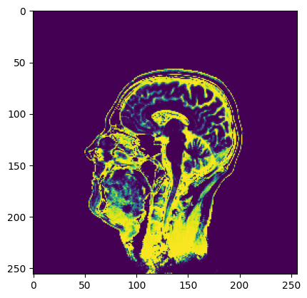
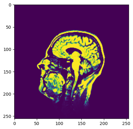
本当はバイアスフィールドを加味してパラメータ(平均値と標準偏差)を更新した方がよいだろう(今回はうまくできなかった)。
収束判定をpatience回数にしているが、abs(current_log_likelifood-prev_log_likelifood)< tolerance のようにした方がベターだろう。
免責
コードの間違いや解釈の違いによる実装の違いが含まれている可能性があります。