pythonによるネットワーク分析のメモ書きとなります。
networkxを使用します。
内容・コードがまとまっていないので、詳細については参考書の参照をお願いします。
機会があればしっかり勉強していこうと思います。
ネットワークの基礎知識
ネットワークは、頂点(ノード)とそれをつなぐ辺(エッジ、リンク)によって構成される。
ネットワークすべての辺を並べて表すデータ構造を辺リストと呼ぶ。
import pandas as pd
import numpy as np

d1 = pd.read_csv('pos.csv', encoding='shift-jis')
import networkx as nx
import matplotlib.pyplot as plt
import japanize_matplotlib
styles = {'node_size':1400,
'font_size':15,
'node_color':'lightblue',
'with_labels':True,
'font_weight':'bold',
'font_family':'MS Gothic'}
# Graphオブジェクトの作成
G1 = nx.Graph()
# nodeデータの追加
nodes1 = np.unique([d.形態素1]+[d.形態素2])
edges1 = [(d.loc[i, '形態素1'], d.loc[i, '形態素2']) for i in range(len(d))]
G1.add_nodes_from(nodes1)
G1.add_edges_from(edges1)
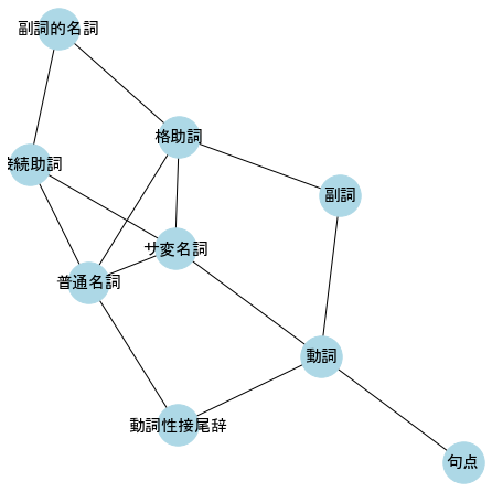
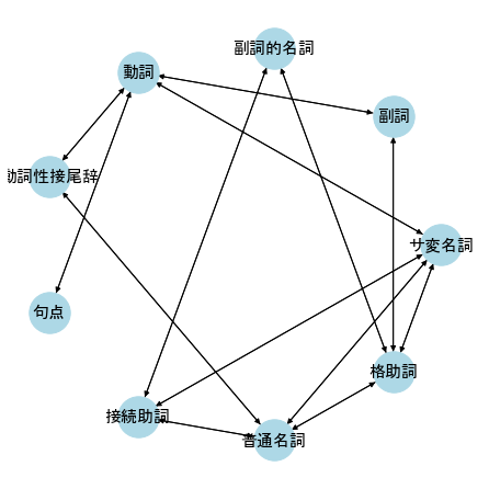
# ネットワークの可視化
plt.figure(figsize=(6,6))
nx.draw(G1, **styles)
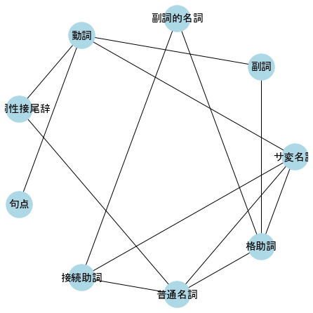
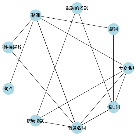
描画方法には様々なものがある。
plt.figure(figsize=(25,8))
# ランダム
plt.subplot(131)
nx.draw_random(G1, **styles)

# 円周上
plt.subplot(132)
nx.draw_circular(G1, **styles)

# ばね配置
plt.subplot(133)
nx.draw_spring(G1, **styles)

頂点の数や頂点のリスト、辺の数や辺のリストは次のように表示される。
print('number of nodes:', G1.number_of_nodes())
print(G1.nodes())
print('number of edges:', G1.number_of_edges())
print(G1.edges())
number of nodes: 9
['サ変名詞', '副詞', '副詞的名詞', '動詞', '動詞性接尾辞', '句点', '接続助詞', '普通名詞', '格助詞']
number of edges: 14
[('サ変名詞', '動詞'), ('サ変名詞', '普通名詞'), ('サ変名詞', '接続助詞'), ('サ変名詞', '格助詞'), ('副詞', '動詞'), ('副詞', '格助詞'), ('副詞的名詞', '格助詞'), ('副詞的名詞', '接続助詞'), ('動詞', '動詞性接尾辞'), ('動詞', '句点'), ('動詞性接尾辞', '動詞性接尾辞'), ('動詞性接尾辞', '普通名詞'), ('接続助詞', '普通名詞'), ('普通名詞', '格助詞')]
ネットワークを表すデータ構造として、隣接行列がよく用いられる。
print('sparse adjacency matrix:')
print(nx.adjacency_matrix(G1))
print('dense adjacency matrix:')
print(nx.adjacency_matrix(G1).todense().astype(int))
sparse adjacency matrix:
  (0, 3)	1.0
  (0, 6)	1.0
  (0, 7)	1.0
  (0, 8)	1.0
  (1, 3)	1.0
  (1, 8)	1.0
  (2, 6)	1.0
  (2, 8)	1.0
  (3, 0)	1.0
  (3, 1)	1.0
  (3, 4)	1.0
  (3, 5)	1.0
  (4, 3)	1.0
  (4, 4)	1.0
  (4, 7)	1.0
  (5, 3)	1.0
  (6, 0)	1.0
  (6, 2)	1.0
  (6, 7)	1.0
  (7, 0)	1.0
  (7, 4)	1.0
  (7, 6)	1.0
  (7, 8)	1.0
  (8, 0)	1.0
  (8, 1)	1.0
  (8, 2)	1.0
  (8, 7)	1.0
dense adjacency matrix:
[[0 0 0 1 0 0 1 1 1]
 [0 0 0 1 0 0 0 0 1]
 [0 0 0 0 0 0 1 0 1]
 [1 1 0 0 1 1 0 0 0]
 [0 0 0 1 1 0 0 1 0]
 [0 0 0 1 0 0 0 0 0]
 [1 0 1 0 0 0 0 1 0]
 [1 0 0 0 1 0 1 0 1]
 [1 1 1 0 0 0 0 1 0]]
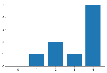
次数
ネットワークの頂点の次数とは、その頂点につながる辺の数を表す。
次数ごとにその時数を持つ頂点数を表したものを次数分布と呼ぶ。
print('degree:',G1.degree())
print(nx.degree_histogram(G1))
print(nx.info(G1))
plt.bar(range(5), height=nx.degree_histogram(G1))
degree: [('サ変名詞', 4), ('副詞', 2), ('副詞的名詞', 2), ('動詞', 4), ('動詞性接尾辞', 4), ('句点', 1), ('接続助詞', 3), ('普通名詞', 4), ('格助詞', 4)]
[0, 1, 2, 1, 5]
Name:
Type: Graph
Number of nodes: 9
Number of edges: 14
Average degree:   3.1111


<BarContainer object of 5 artists>
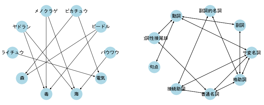
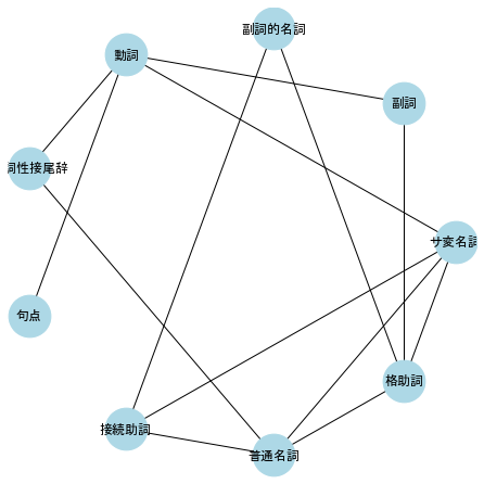
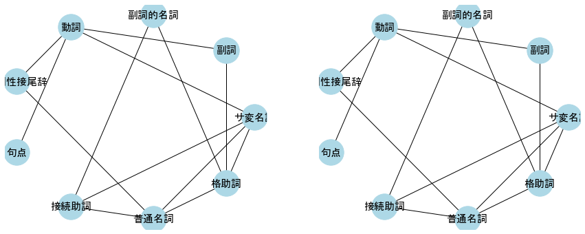
有向グラフ・無向グラフ
ネットワークの辺に向きがあるものを有向グラフ、ないものを無向グラフと呼ぶ。
有向グラフでは、辺に向きがあるため頂点に入ってくる入次数と、頂点から出ていく出次数の2つがある。
# Graphオブジェクトの作成
G1 = nx.Graph()

# nodeデータの追加
v = np.unique([d1.形態素1]+[d1.形態素2])
G1.add_nodes_from(v)

# edgeデータの追加
G1.add_edges_from([(d1.loc[i, '形態素1'], d1.loc[i, '形態素2']) for i in range(len(d1))])

# ネットワークの可視化
plt.figure(figsize=(6,6))
nx.draw_circular(G1, **styles)

print(nx.info(G1))
Name:
Type: Graph
Number of nodes: 9
Number of edges: 14
Average degree:   3.1111
# Graphオブジェクトの作成
DG1 = nx.DiGraph(G1)

plt.figure(figsize=(6,6))
nx.draw_circular(DG1, **styles)

print(nx.info(DG1))
Name:
Type: DiGraph
Number of nodes: 9
Number of edges: 27
Average in degree:   3.0000
Average out degree:   3.0000

多重辺、自己ループ
2点間をつなぐ複数の辺を多重辺、同一頂点を結ぶ辺を自己ループと呼ぶ。
d2 = pd.concat([d1, pd.DataFrame({'形態素1':['普通名詞','普通名詞','普通名詞'],
                                  '形態素2':['普通名詞','動詞','動詞'],
                                  '共起':[1,2,1]})]).reset_index(drop=False)
d2
| index | 形態素1 | 形態素2 | 共起 | |
|---|---|---|---|---|
| 0 | 0 | 普通名詞 | 接続助詞 | 2 |
| 1 | 1 | 普通名詞 | 格助詞 | 2 |
| 2 | 2 | サ変名詞 | 動詞 | 1 |
| 3 | 3 | サ変名詞 | 普通名詞 | 1 |
| 4 | 4 | 副詞 | 動詞 | 1 |
| 5 | 5 | 副詞的名詞 | 格助詞 | 1 |
| 6 | 6 | 動詞 | 動詞性接尾辞 | 1 |
| 7 | 7 | 動詞 | 句点 | 1 |
| 8 | 8 | 動詞性接尾辞 | 動詞性接尾辞 | 1 |
| 9 | 9 | 動詞性接尾辞 | 普通名詞 | 1 |
| 10 | 10 | 接続助詞 | サ変名詞 | 1 |
| 11 | 11 | 接続助詞 | 副詞的名詞 | 1 |
| 12 | 12 | 格助詞 | サ変名詞 | 1 |
| 13 | 13 | 格助詞 | 副詞 | 1 |
| 14 | 14 | 格助詞 | 普通名詞 | 1 |
| 15 | 0 | 普通名詞 | 普通名詞 | 1 |
| 16 | 1 | 普通名詞 | 動詞 | 2 |
| 17 | 2 | 普通名詞 | 動詞 | 1 |
nodes2 = np.unique([d2.形態素1]+[d2.形態素2])
edges2 = [(d2.loc[i, '形態素1'], d2.loc[i, '形態素2']) for i in range(len(d2))]

MG1 = nx.MultiGraph()
MG1.add_nodes_from(nodes2)
MG1.add_edges_from(edges2)

# ネットワークの可視化
plt.figure(figsize=(6,6))
nx.draw_circular(MG1, **styles)

print('degree:', MG1.degree())
print(nx.info(MG1))
degree: [('サ変名詞', 4), ('副詞', 2), ('副詞的名詞', 2), ('動詞', 6), ('動詞性接尾辞', 4), ('句点', 1), ('接続助詞', 3), ('普通名詞', 9), ('格助詞', 5)]
Name:
Type: MultiGraph
Number of nodes: 9
Number of edges: 18
Average degree:   4.0000
2部グラフ
2種類の頂点から構成され、異なる種類の頂点にしか間にしか辺が存在しないグラフを2部グラフと呼ぶ。
「論文とその著者」など。
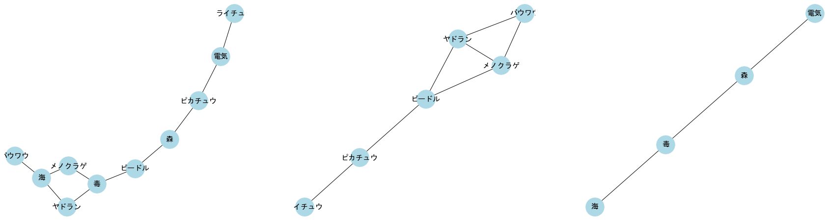
2部グラフから同一種類の頂点のグラフを生成する方法として、プロジェクションがある。
もとの2部グラフにおいて、距離2でつながっている頂点を辺で結んだグラフを生成するものである。
pokemon1 = pd.DataFrame({'ポケモン':['ピカチュウ','ピカチュウ','ライチュウ','ビードル','ビードル','メノクラゲ','メノクラゲ','ヤドラン','ヤドラン','パウワウ'],
                        '図鑑単語':['森','電気','電気','森','毒','海','毒','海','毒','海']})
pokemon1
| ポケモン | 図鑑単語 | |
|---|---|---|
| 0 | ピカチュウ | 森 |
| 1 | ピカチュウ | 電気 |
| 2 | ライチュウ | 電気 |
| 3 | ビードル | 森 |
| 4 | ビードル | 毒 |
| 5 | メノクラゲ | 海 |
| 6 | メノクラゲ | 毒 |
| 7 | ヤドラン | 海 |
| 8 | ヤドラン | 毒 |
| 9 | パウワウ | 海 |
from networkx.algorithms import bipartite

B1 = nx.Graph()
B1.add_nodes_from(list(np.unique(pokemon1['ポケモン'])), bipartite=0)
B1.add_nodes_from(list(np.unique(pokemon1['図鑑単語'])), bipartite=1)
B1.add_edges_from([(pokemon1.loc[i, 'ポケモン'], pokemon1.loc[i, '図鑑単語']) for i in range(len(pokemon))])

plt.figure(figsize=(30,8))
plt.subplot(131)
nx.draw(B1, **styles)

top_nodes = set(n for n, d in B1.nodes(data=True) if d['bipartite']==0)
bottom_nodes = set(B1) - top_nodes
print('top nodes :',top_nodes)
print('bottom nodes :',bottom_nodes)

GT = bipartite.projected_graph(B1, top_nodes)
print('projected graph (top nodes):', GT.edges())

plt.subplot(132)
nx.draw(GT, **styles)

GB = bipartite.projected_graph(B1, bottom_nodes)
print('projected graph (bottom nodes):', GB.edges())

plt.subplot(133)
nx.draw(GB, **styles)
top nodes : {'ピカチュウ', 'ヤドラン', 'ビードル', 'ライチュウ', 'パウワウ', 'メノクラゲ'}
bottom nodes : {'毒', '電気', '海', '森'}
projected graph (top nodes): [('ピカチュウ', 'ビードル'), ('ピカチュウ', 'ライチュウ'), ('ヤドラン', 'パウワウ'), ('ヤドラン', 'ビードル'), ('ヤドラン', 'メノクラゲ'), ('ビードル', 'メノクラゲ'), ('パウワウ', 'メノクラゲ')]
projected graph (bottom nodes): [('毒', '海'), ('毒', '森'), ('電気', '森')]
パス
頂点Aと辺でつながっている他の頂点に移ることを繰り返して、最終的にBに到着したとき、この辺の集合を頂点と頂点Bの間のパスと呼ぶ。
また、パスの中の辺の数をパスの長さと呼ぶ。
2頂点間の長さ$r$のパスの有無は隣接行列の積によって求めることができる。
長さ2の場合は$A^2$、長さ3の場合は$A^3$となる。
# ネットワークの可視化
plt.figure(figsize=(6,6))
nx.draw_circular(G1, node_size=1500, node_color='lightblue', with_labels=True, font_family='MS Gothic')

Z = nx.adjacency_matrix(G).todense().astype(int)
print('adjacency matrix A:')
print(Z)
print('A*A:')
print(Z**2)
print('degree:', G.degree())
print('A*A*A')
print(Z**3)
adjacency matrix A:
[[0 0 0 1 0 0 1 1 1]
 [0 0 0 1 0 0 0 0 1]
 [0 0 0 0 0 0 1 0 1]
 [1 1 0 0 1 1 0 0 0]
 [0 0 0 1 1 0 0 1 0]
 [0 0 0 1 0 0 0 0 0]
 [1 0 1 0 0 0 0 1 0]
 [1 0 0 0 1 0 1 0 1]
 [1 1 1 0 0 0 0 1 0]]
A*A:
[[4 2 2 0 2 1 1 2 1]
 [2 2 1 0 1 1 0 1 0]
 [2 1 2 0 0 0 0 2 0]
 [0 0 0 4 1 0 1 2 2]
 [2 1 0 1 3 1 1 1 1]
 [1 1 0 0 1 1 0 0 0]
 [1 0 0 1 1 0 3 1 3]
 [2 1 2 2 1 0 1 4 1]
 [1 0 0 2 1 0 3 1 4]]
degree: [('サ変名詞', 4), ('副詞', 2), ('副詞的名詞', 2), ('動詞', 4), ('動詞性接尾辞', 4), ('句点', 1), ('接続助詞', 3), ('普通名詞', 4), ('格助詞', 4)]
A*A*A
[[ 4  1  2  9  4  0  8  8 10]
 [ 1  0  0  6  2  0  4  3  6]
 [ 2  0  0  3  2  0  6  2  7]
 [ 9  6  3  1  7  4  2  4  2]
 [ 4  2  2  7  5  1  3  7  4]
 [ 0  0  0  4  1  0  1  2  2]
 [ 8  4  6  2  3  1  2  8  2]
 [ 8  3  2  4  7  2  8  5  9]
 [10  6  7  2  4  2  2  9  2]]
サイクル
サイクルとは、始点と終点が同一頂点となるパスのことである。
# ネットワークの可視化
plt.figure(figsize=(6,6))
nx.draw_circular(DG1, **styles)

print(nx.info(DG1))

Z = nx.adjacency_matrix(DG1).todense().astype(int)
print('A: = ', np.diag(Z))
print(Z)
print('A*A: diag = ', np.diag(Z**1))
print(Z**2)
print('A*A*A = ', np.diag(Z**3))
print(Z**3)
print('A*A*A*A = ', np.diag(Z**4))
print(Z**4)
Name:
Type: DiGraph
Number of nodes: 9
Number of edges: 27
Average in degree:   3.0000
Average out degree:   3.0000
A: =  [0 0 0 0 1 0 0 0 0]
[[0 0 0 1 0 0 1 1 1]
 [0 0 0 1 0 0 0 0 1]
 [0 0 0 0 0 0 1 0 1]
 [1 1 0 0 1 1 0 0 0]
 [0 0 0 1 1 0 0 1 0]
 [0 0 0 1 0 0 0 0 0]
 [1 0 1 0 0 0 0 1 0]
 [1 0 0 0 1 0 1 0 1]
 [1 1 1 0 0 0 0 1 0]]
A*A: diag =  [0 0 0 0 1 0 0 0 0]
[[4 2 2 0 2 1 1 2 1]
 [2 2 1 0 1 1 0 1 0]
 [2 1 2 0 0 0 0 2 0]
 [0 0 0 4 1 0 1 2 2]
 [2 1 0 1 3 1 1 1 1]
 [1 1 0 0 1 1 0 0 0]
 [1 0 0 1 1 0 3 1 3]
 [2 1 2 2 1 0 1 4 1]
 [1 0 0 2 1 0 3 1 4]]
A*A*A =  [4 0 0 1 5 0 2 5 2]
[[ 4  1  2  9  4  0  8  8 10]
 [ 1  0  0  6  2  0  4  3  6]
 [ 2  0  0  3  2  0  6  2  7]
 [ 9  6  3  1  7  4  2  4  2]
 [ 4  2  2  7  5  1  3  7  4]
 [ 0  0  0  4  1  0  1  2  2]
 [ 8  4  6  2  3  1  2  8  2]
 [ 8  3  2  4  7  2  8  5  9]
 [10  6  7  2  4  2  2  9  2]]
A*A*A*A =  [35 12 13 26 19  4 22 32 32]
[[35 19 18  9 21  9 14 26 15]
 [19 12 10  3 11  6  4 13  4]
 [18 10 13  4  7  3  4 17  4]
 [ 9  3  4 26 12  1 16 20 22]
 [21 11  7 12 19  7 13 16 15]
 [ 9  6  3  1  7  4  2  4  2]
 [14  4  4 16 13  2 22 15 26]
 [26 13 17 20 16  4 15 32 18]
 [15  4  4 22 15  2 26 18 32]]

非循環サイクル
サイクルが存在しないサイクルを、非循環サイクルと呼ぶ。
非循環サイクルであれば、その隣接行列のすべての固有値はゼロであり、その逆も真である。
import numpy.linalg as LA

# Graphオブジェクトの作成
DG2 = nx.DiGraph()

# nodeデータの追加
nodes3 = np.unique([pokemon1.ポケモン]+[pokemon1.図鑑単語])
edges3 = [(pokemon1.loc[i, 'ポケモン'], pokemon1.loc[i, '図鑑単語']) for i in range(len(pokemon1))]

DG2.add_nodes_from(nodes3)
DG2.add_edges_from(edges3)

plt.figure(figsize=(15,6))
plt.subplot(121)
nx.draw_circular(DG2, **styles)

plt.subplot(122)
nx.draw_circular(DG1, **styles)

Z = nx.adjacency_matrix(DG2).todense().astype(int)
w, v = LA.eig(Z)
print('cyclic: eigenvalues =', w)
print(Z)

ZA = nx.adjacency_matrix(DG1).todense().astype(int)
wa, va = LA.eig(ZA)
print('cyclic: eigenvalues =', wa)
print(ZA)
cyclic: eigenvalues = [0.000000 0.000000 0.000000 0.000000 0.000000 0.000000 0.000000 0.000000
 0.000000 0.000000]
[[0 0 0 0 0 0 0 0 1 0]
 [0 0 0 0 0 0 1 1 0 0]
 [0 0 0 0 0 0 1 0 0 1]
 [0 0 0 0 0 0 0 1 1 0]
 [0 0 0 0 0 0 0 1 1 0]
 [0 0 0 0 0 0 0 0 0 1]
 [0 0 0 0 0 0 0 0 0 0]
 [0 0 0 0 0 0 0 0 0 0]
 [0 0 0 0 0 0 0 0 0 0]
 [0 0 0 0 0 0 0 0 0 0]]
cyclic: eigenvalues = [3.353269 -2.546447 -1.996967 1.711009 1.098629 -0.840992 0.470910
 0.182422 -0.431834]
[[0 0 0 1 0 0 1 1 1]
 [0 0 0 1 0 0 0 0 1]
 [0 0 0 0 0 0 1 0 1]
 [1 1 0 0 1 1 0 0 0]
 [0 0 0 1 1 0 0 1 0]
 [0 0 0 1 0 0 0 0 0]
 [1 0 1 0 0 0 0 1 0]
 [1 0 0 0 1 0 1 0 1]
 [1 1 1 0 0 0 0 1 0]]
サイクルがない有向グラフはDAGと呼ばれる。DAGは隣接行列の行と列を入れ替えることで三角行列にすることができる。
無向でサイクルがないグラフは木や森と呼ばれる。木において頂点の数$n$、辺の数$m$とすると$n=m+1$となる。
直径
グラフにおける直径とは、グラフの任意の2頂点間における最短パス長の中で、最大のもののことをいう。
# ネットワークの可視化
plt.figure(figsize=(6,6))
nx.draw_circular(G1, node_size=1500, node_color='lightblue', with_labels=True, font_family='MS Gothic')

Z = nx.adjacency_matrix(G1).todense().astype(int)
print('shortest path between 句点 and 副詞的名詞:',nx.shortest_path(G1, "句点", '副詞的名詞'))
print('all shortest paths:', [p for p in nx.all_shortest_paths(G1, "句点", '副詞的名詞')])
print('shortest path length:', nx.shortest_path_length(G1, "句点", '副詞的名詞'))
print('diameter:', nx.diameter(G1))
shortest path between 句点 and 副詞的名詞: ['句点', '動詞', 'サ変名詞', '格助詞', '副詞的名詞']
all shortest paths: [['句点', '動詞', 'サ変名詞', '接続助詞', '副詞的名詞'], ['句点', '動詞', 'サ変名詞', '格助詞', '副詞的名詞'], ['句点', '動詞', '副詞', '格助詞', '副詞的名詞']]
shortest path length: 4
diameter: 4
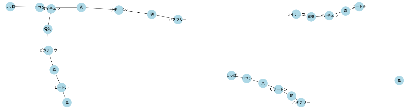
連結成分
連結、連結成分
グラフ上の2頂点間のパスが存在するとき、そのグラフは連結であるという。
また、任意の2頂点間のパスが存在するような部分グラフを、そのグラフの連結成分と呼ぶ。
連結成分の個数は、グラフラプラシアンの固有値がゼロとなるものの個数で求められる。
グラフラプラシアンとは、グラフの隣接行列を$A$、各頂点の次数を対角成分に持つ対角ベクトルを$D$としたとき,$L=D-A$で求められる行列である。
pokemon2 = pd.DataFrame({'ポケモン':['ピカチュウ','ピカチュウ','ライチュウ','ビードル','ビードル','メノクラゲ','メノクラゲ','ヤドラン','ヤドラン','パウワウ'],
                        '図鑑単語':['森','電気','電気','森','毒','海','毒','海','毒','海']})
pokemon2
| ポケモン | 図鑑単語 | |
|---|---|---|
| 0 | ピカチュウ | 森 |
| 1 | ピカチュウ | 電気 |
| 2 | ライチュウ | 電気 |
| 3 | ビードル | 森 |
| 4 | ビードル | 毒 |
| 5 | メノクラゲ | 海 |
| 6 | メノクラゲ | 毒 |
| 7 | ヤドラン | 海 |
| 8 | ヤドラン | 毒 |
| 9 | パウワウ | 海 |
from networkx.algorithms import bipartite

B2 = nx.Graph()
B2.add_nodes_from(list(np.unique(pokemon2['ポケモン'])), bipartite=0)
B2.add_nodes_from(list(np.unique(pokemon2['図鑑単語'])), bipartite=1)
B2.add_edges_from([(pokemon2.loc[i, 'ポケモン'], pokemon2.loc[i, '図鑑単語']) for i in range(len(pokemon))])

plt.figure(figsize=(30,8))
plt.subplot(121)
nx.draw(B2, **styles)

print('connected')
print('number of connected components:', nx.number_connected_components(B2))
L = nx.laplacian_matrix(B2).todense().astype(int)
print('Laplacian matrix L:')
print(L)
np.set_printoptions(formatter={'float':'{:3f}'.format})
print('eigenvalues of L', LA.eigvals(L))

print('disconnected')
B2.remove_edges_from([('ビードル','毒')])

plt.subplot(122)
nx.draw(B2, **styles)

print('number of connected components:', nx.number_connected_components(B2))
L = nx.laplacian_matrix(B2).todense().astype(int)
print('Laplacian matrix L:')
print(L)
print('eigenvalues of L', LA.eigvals(L))
connected
number of connected components: 2
Laplacian matrix L:
[[ 1  0  0  0  0  0  0  0  0  0 -1  0]
 [ 0  2  0  0  0  0  0 -1 -1  0  0  0]
 [ 0  0  2  0  0  0  0 -1  0  0  0 -1]
 [ 0  0  0  1  0  0  0  0  0  0  0 -1]
 [ 0  0  0  0  2  0  0  0  0 -1 -1  0]
 [ 0  0  0  0  0  2 -1  0  0 -1  0  0]
 [ 0  0  0  0  0 -1  1  0  0  0  0  0]
 [ 0 -1 -1  0  0  0  0  2  0  0  0  0]
 [ 0 -1  0  0  0  0  0  0  1  0  0  0]
 [ 0  0  0  0 -1 -1  0  0  0  2  0  0]
 [-1  0  0  0 -1  0  0  0  0  0  2  0]
 [ 0  0 -1 -1  0  0  0  0  0  0  0  2]]
eigenvalues of L [3.732051 3.000000 2.000000 1.000000 0.000000 0.267949 3.732051 3.000000
 2.000000 1.000000 -0.000000 0.267949]
disconnected
number of connected components: 2
Laplacian matrix L:
[[ 1  0  0  0  0  0  0  0  0  0 -1  0]
 [ 0  2  0  0  0  0  0 -1 -1  0  0  0]
 [ 0  0  2  0  0  0  0 -1  0  0  0 -1]
 [ 0  0  0  1  0  0  0  0  0  0  0 -1]
 [ 0  0  0  0  2  0  0  0  0 -1 -1  0]
 [ 0  0  0  0  0  2 -1  0  0 -1  0  0]
 [ 0  0  0  0  0 -1  1  0  0  0  0  0]
 [ 0 -1 -1  0  0  0  0  2  0  0  0  0]
 [ 0 -1  0  0  0  0  0  0  1  0  0  0]
 [ 0  0  0  0 -1 -1  0  0  0  2  0  0]
 [-1  0  0  0 -1  0  0  0  0  0  2  0]
 [ 0  0 -1 -1  0  0  0  0  0  0  0  2]]
eigenvalues of L [3.732051 3.000000 2.000000 1.000000 0.000000 0.267949 3.732051 3.000000
 2.000000 1.000000 -0.000000 0.267949]
強連結成分
有向グラフにおいて、任意の2頂点間のパスが存在するような部分グラフを、そのグラフの強連結成分(SCC)と呼ぶ。
# ネットワークの可視化
plt.figure(figsize=(6,6))
nx.draw_circular(DG1, **styles)

print('number of strogly connected components:', nx.number_strongly_connected_components(DG1))
number of strogly connected components: 1
ある頂点$A$から到達可能な頂点集合を「頂点$A$のout-components」、
頂点$A$に到達可能な頂点の集合を「頂点$A$のin-components」と呼ぶ。
連結性
2頂点間のパスの数を連結性と呼ぶ。
for path in nx.all_simple_paths(DG1, "接続助詞", '動詞'):
    print(path)

print('shortest path length from 接続助詞 to 動詞:', nx.shortest_path_length(DG1, "接続助詞", '動詞'))
print('shortest path from 接続助詞 to 動詞:', nx.shortest_path(DG1, "接続助詞", '動詞'))
['接続助詞', '普通名詞', '格助詞', 'サ変名詞', '動詞']
['接続助詞', '普通名詞', '格助詞', '副詞', '動詞']
['接続助詞', '普通名詞', 'サ変名詞', '動詞']
['接続助詞', '普通名詞', 'サ変名詞', '格助詞', '副詞', '動詞']
['接続助詞', '普通名詞', '動詞性接尾辞', '動詞']
['接続助詞', 'サ変名詞', '動詞']
['接続助詞', 'サ変名詞', '普通名詞', '格助詞', '副詞', '動詞']
['接続助詞', 'サ変名詞', '普通名詞', '動詞性接尾辞', '動詞']
['接続助詞', 'サ変名詞', '格助詞', '普通名詞', '動詞性接尾辞', '動詞']
['接続助詞', 'サ変名詞', '格助詞', '副詞', '動詞']
['接続助詞', '副詞的名詞', '格助詞', '普通名詞', 'サ変名詞', '動詞']
['接続助詞', '副詞的名詞', '格助詞', '普通名詞', '動詞性接尾辞', '動詞']
['接続助詞', '副詞的名詞', '格助詞', 'サ変名詞', '動詞']
['接続助詞', '副詞的名詞', '格助詞', 'サ変名詞', '普通名詞', '動詞性接尾辞', '動詞']
['接続助詞', '副詞的名詞', '格助詞', '副詞', '動詞']
shortest path length from 接続助詞 to 動詞: 2
shortest path from 接続助詞 to 動詞: ['接続助詞', 'サ変名詞', '動詞']
2頂点間の辺カット集合とは、集合内の辺を除去することで、その2頂点間が非連結になるような集合を指す。
そのような集合で、最小のものを最小カットと呼ぶ。最大流とは、2頂点間のパスの数を指す。
最大流最小カットは、この両者が等しいことを示す定理であり、各辺の容量が異なっている場合でも成立する。
from pprint import pprint

# Graphオブジェクトの作成
G1 = nx.Graph()
G1.add_nodes_from(nodes1)
G1.add_edges_from(edges1, capacity=1.0)

capa = nx.get_edge_attributes(G1, 'capacity')
print(capa)

plt.figure(figsize=(15,6))
plt.subplot(121)
nx.draw_circular(G1, **styles)

cut_deges = nx.algorithms.connectivity.minimum_edge_cut(G1, "動詞", "普通名詞")
print('cut size of 動詞 and 普通名詞', cut_deges)
flow_value, floe_dict = nx.algorithms.flow.maximum_flow(G1, "動詞", "普通名詞")
print('max flow of 動詞 and 普通名詞', flow_value)

print('edge 動詞-動詞性接尾辞 is deleted')
G.remove_edges_from([('動詞','動詞性接尾辞')])

plt.subplot(122)
nx.draw_circular(G1, **styles)

cut_deges = nx.algorithms.connectivity.minimum_edge_cut(G1, "動詞", "普通名詞")
print('cut size of 動詞 and 普通名詞', cut_deges)
flow_value, floe_dict = nx.algorithms.flow.maximum_flow(G1, "動詞", "普通名詞")
print('max flow of 動詞 and 普通名詞', flow_value)
{('サ変名詞', '動詞'): 1.0, ('サ変名詞', '普通名詞'): 1.0, ('サ変名詞', '接続助詞'): 1.0, ('サ変名詞', '格助詞'): 1.0, ('副詞', '動詞'): 1.0, ('副詞', '格助詞'): 1.0, ('副詞的名詞', '格助詞'): 1.0, ('副詞的名詞', '接続助詞'): 1.0, ('動詞', '動詞性接尾辞'): 1.0, ('動詞', '句点'): 1.0, ('動詞性接尾辞', '動詞性接尾辞'): 1.0, ('動詞性接尾辞', '普通名詞'): 1.0, ('接続助詞', '普通名詞'): 1.0, ('普通名詞', '格助詞'): 1.0}
cut size of 動詞 and 普通名詞 {('動詞', 'サ変名詞'), ('動詞性接尾辞', '普通名詞'), ('副詞', '格助詞')}
max flow of 動詞 and 普通名詞 3.0
edge 動詞-動詞性接尾辞 is deleted
cut size of 動詞 and 普通名詞 {('動詞', 'サ変名詞'), ('動詞性接尾辞', '普通名詞'), ('副詞', '格助詞')}
max flow of 動詞 and 普通名詞 3.0
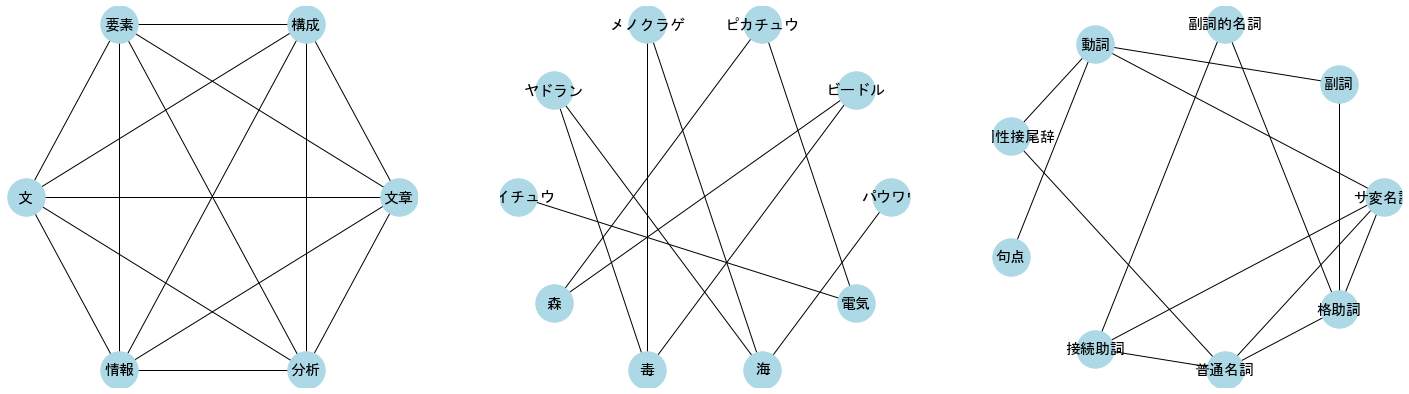
クラスタ係数
クラスタ係数は例えば「ある人の2人の友人が友人同士である割合」を表す。
local clustering coefficient
頂点$i$の次数を$k_i$としたとき、頂点$i$の友人のペア総数は$k_i(k_i-1)/2$あり、その中で辺で結ばれたものの割合を、頂点$i$に関するクラスタ係数$C_i$と呼ぶ。
頂点$i$の隣接頂点間のつながり具合を表す指標としてredundancy($R_i$)がある。これは頂点$i$の隣接頂点について、頂点$i$の他の隣接頂点と辺でつながっているものの数の平均である。
「頂点$i$の友人ペアの中で辺で結ばれたものの数」は$k_iR_i/2$であるから、$C_i$は次のように表せる。
C_i=\frac{k_iR_i/2}{k_i(k_i-1)/2}=\frac{R_i}{k_i-1}
$C_i$をネットワークすべての頂点で平均を取った$C_{WS}=\frac{1}{n}\sum_i^nC_i$をネットワーク全体のクラスタ係数と呼ぶ。
完全グラフのクラスタ係数は1、2部グラフのクラスタ係数は0、ランダムグラフのクラスタ係数は0から1の間の数となる。
d3 = pd.read_csv('co_occur.csv', encoding='shift-jis')

G3 = nx.Graph()
G3.add_edges_from([(d3.loc[i, '語1'], d3.loc[i, '語2']) for i in range(len(d3))], capacity=1.0)
G3.add_weighted_edges_from([(d3.loc[i, '語1'], d3.loc[i, '語2'], d3.loc[i, 'Freq']) for i in range(len(d1))])

plt.figure(figsize=(25,7))

plt.subplot(131)
nx.draw_circular(G3, **styles)

plt.subplot(132)
nx.draw_circular(B1, **styles)

plt.subplot(133)
nx.draw_circular(G1, **styles)

print('CC of complete graph', nx.clustering(G3, '文章'))
print('CC of bipartite graph', nx.clustering(B1, 'ピカチュウ'))
print('CC of random graph', nx.clustering(G1, '格助詞'))
CC of complete graph 1.0
CC of bipartite graph 0
CC of random graph 0.16666666666666666
クラスタ係数のもう一つの定義は、「ネットワーク全体における長さ2のパス$N^{(2)}$のなかで、そのパスが閉路となるものの割合」である。
三角形の個数を$L_3$とすると、3頂点からなる三角形1つは、長さ2のパスで閉路となるもの6つに対応するので$C=\frac{6L_3}{|N^{(2)}|}$となる。
参考文献