Pythonを用いて格子ボルツマン法を試行

pythonを用いて格子ボルツマン法

格子ボルツマン法とは何かはさておき、シミュレーションしてから理解するという所謂「形から入る」という手段をとる。
こちらのURLを参考にする。
http://physics.weber.edu/schroeder/fluids/

目的

とりあえず数値計算を実行してみる。
URLにはドキュメントもあり（英文だが）、そちらは別途コードの解説と合わせて投稿しようと思う。

環境

windows10
python3.6.4
(コマンドプロンプトからpythonを起動)

(1)pythonのインストール
https://qiita.com/taiponrock/items/f574dd2cddf8851fb02c

外部ライブラリのインストール

以下のものがインストールされていれば、コマンドプロンプトから計算が実行できる。

(2)numpyのインストール
https://qiita.com/kenichi-t/items/7319b3876ae7f0d3817c
(3)matplotlibのインストール
https://qiita.com/Morio/items/d75159bac916174e7654

pythonコード

URLのpythonコードは2系で書かれている。python3.6.4(python3系)で実行するためには、少し修正が必要である。
python2系を扱ったことがないので、詳しくは知らないが以下の修正を行うことで正常に計算実行できる。

その1

barrier[(height/2)-8:(height/2)+8, (height/2)] = True

これでは配列部分が実数になるので、以下のように整数型になるように修正する必要がある。
【修正】
barrier[int(height/2)-8:int(height/2)+8, int(height/2)] = True


その2

print "%1.1f" % (100/(endTime-startTime)), 'frames per second'

これはpython2系の書き方である。python3系では以下ののように（）でくくる必要がある。
【修正】
print ("%1.1f" % (100/(endTime-startTime)), 'frames per second')


修正が終わったので、コマンドプロンプトを起動して、以下をタイプして計算実行。
※ファイルの保存の際は、文字コードはUTF-8を選択

python Lattice_Boltzman.py


サンプルコードは以下に示す（余計なコメントが多かったので、シンプルにした）

Lattice_Boltzman.py

import numpy
import time
import matplotlib.pyplot
import matplotlib.animation

# Define constants:
height = 80                         # lattice dimensions
width = 200
viscosity = 0.02                    # fluid viscosity
omega = 1 / (3*viscosity + 0.5)     # "relaxation" parameter
u0 = 0.1                            # initial and in-flow speed
four9ths = 4.0/9.0                  # abbreviations for lattice-Boltzmann weight factors
one9th   = 1.0/9.0
one36th  = 1.0/36.0
performanceData = False             # set to True if performance data is desired

# Initialize all the arrays to steady rightward flow:
n0 = four9ths * (numpy.ones((height,width)) - 1.5*u0**2)    # particle densities along 9 directions
nN = one9th * (numpy.ones((height,width)) - 1.5*u0**2)
nS = one9th * (numpy.ones((height,width)) - 1.5*u0**2)
nE = one9th * (numpy.ones((height,width)) + 3*u0 + 4.5*u0**2 - 1.5*u0**2)
nW = one9th * (numpy.ones((height,width)) - 3*u0 + 4.5*u0**2 - 1.5*u0**2)
nNE = one36th * (numpy.ones((height,width)) + 3*u0 + 4.5*u0**2 - 1.5*u0**2)
nSE = one36th * (numpy.ones((height,width)) + 3*u0 + 4.5*u0**2 - 1.5*u0**2)
nNW = one36th * (numpy.ones((height,width)) - 3*u0 + 4.5*u0**2 - 1.5*u0**2)
nSW = one36th * (numpy.ones((height,width)) - 3*u0 + 4.5*u0**2 - 1.5*u0**2)
rho = n0 + nN + nS + nE + nW + nNE + nSE + nNW + nSW        # macroscopic density
ux = (nE + nNE + nSE - nW - nNW - nSW) / rho                # macroscopic x velocity
uy = (nN + nNE + nNW - nS - nSE - nSW) / rho                # macroscopic y velocity

# Initialize barriers:
barrier = numpy.zeros((height,width), bool)                 # True wherever there's a barrier
barrier[int(height/2)-8:int(height/2)+8, int(height/2)] = True          # simple linear barrier
barrierN = numpy.roll(barrier,  1, axis=0)                  # sites just north of barriers
barrierS = numpy.roll(barrier, -1, axis=0)                  # sites just south of barriers
barrierE = numpy.roll(barrier,  1, axis=1)                  # etc.
barrierW = numpy.roll(barrier, -1, axis=1)
barrierNE = numpy.roll(barrierN,  1, axis=1)
barrierNW = numpy.roll(barrierN, -1, axis=1)
barrierSE = numpy.roll(barrierS,  1, axis=1)
barrierSW = numpy.roll(barrierS, -1, axis=1)

# Move all particles by one step along their directions of motion (pbc):
def stream():
    global nN, nS, nE, nW, nNE, nNW, nSE, nSW
    nN  = numpy.roll(nN,   1, axis=0)   # axis 0 is north-south; + direction is north
    nNE = numpy.roll(nNE,  1, axis=0)
    nNW = numpy.roll(nNW,  1, axis=0)
    nS  = numpy.roll(nS,  -1, axis=0)
    nSE = numpy.roll(nSE, -1, axis=0)
    nSW = numpy.roll(nSW, -1, axis=0)
    nE  = numpy.roll(nE,   1, axis=1)   # axis 1 is east-west; + direction is east
    nNE = numpy.roll(nNE,  1, axis=1)
    nSE = numpy.roll(nSE,  1, axis=1)
    nW  = numpy.roll(nW,  -1, axis=1)
    nNW = numpy.roll(nNW, -1, axis=1)
    nSW = numpy.roll(nSW, -1, axis=1)
    # Use tricky boolean arrays to handle barrier collisions (bounce-back):
    nN[barrierN] = nS[barrier]
    nS[barrierS] = nN[barrier]
    nE[barrierE] = nW[barrier]
    nW[barrierW] = nE[barrier]
    nNE[barrierNE] = nSW[barrier]
    nNW[barrierNW] = nSE[barrier]
    nSE[barrierSE] = nNW[barrier]
    nSW[barrierSW] = nNE[barrier]

# Collide particles within each cell to redistribute velocities (could be optimized a little more):
def collide():
    global rho, ux, uy, n0, nN, nS, nE, nW, nNE, nNW, nSE, nSW
    rho = n0 + nN + nS + nE + nW + nNE + nSE + nNW + nSW
    ux = (nE + nNE + nSE - nW - nNW - nSW) / rho
    uy = (nN + nNE + nNW - nS - nSE - nSW) / rho
    ux2 = ux * ux               # pre-compute terms used repeatedly...
    uy2 = uy * uy
    u2 = ux2 + uy2
    omu215 = 1 - 1.5*u2         # "one minus u2 times 1.5"
    uxuy = ux * uy
    n0 = (1-omega)*n0 + omega * four9ths * rho * omu215
    nN = (1-omega)*nN + omega * one9th * rho * (omu215 + 3*uy + 4.5*uy2)
    nS = (1-omega)*nS + omega * one9th * rho * (omu215 - 3*uy + 4.5*uy2)
    nE = (1-omega)*nE + omega * one9th * rho * (omu215 + 3*ux + 4.5*ux2)
    nW = (1-omega)*nW + omega * one9th * rho * (omu215 - 3*ux + 4.5*ux2)
    nNE = (1-omega)*nNE + omega * one36th * rho * (omu215 + 3*(ux+uy) + 4.5*(u2+2*uxuy))
    nNW = (1-omega)*nNW + omega * one36th * rho * (omu215 + 3*(-ux+uy) + 4.5*(u2-2*uxuy))
    nSE = (1-omega)*nSE + omega * one36th * rho * (omu215 + 3*(ux-uy) + 4.5*(u2-2*uxuy))
    nSW = (1-omega)*nSW + omega * one36th * rho * (omu215 + 3*(-ux-uy) + 4.5*(u2+2*uxuy))
    # Force steady rightward flow at ends (no need to set 0, N, and S components):
    nE[:,0] = one9th * (1 + 3*u0 + 4.5*u0**2 - 1.5*u0**2)
    nW[:,0] = one9th * (1 - 3*u0 + 4.5*u0**2 - 1.5*u0**2)
    nNE[:,0] = one36th * (1 + 3*u0 + 4.5*u0**2 - 1.5*u0**2)
    nSE[:,0] = one36th * (1 + 3*u0 + 4.5*u0**2 - 1.5*u0**2)
    nNW[:,0] = one36th * (1 - 3*u0 + 4.5*u0**2 - 1.5*u0**2)
    nSW[:,0] = one36th * (1 - 3*u0 + 4.5*u0**2 - 1.5*u0**2)

# Compute curl of the macroscopic velocity field:
def curl(ux, uy):
    return numpy.roll(uy,-1,axis=1) - numpy.roll(uy,1,axis=1) - numpy.roll(ux,-1,axis=0) + numpy.roll(ux,1,axis=0)

# Here comes the graphics and animation...
theFig = matplotlib.pyplot.figure(figsize=(8,3))
fluidImage = matplotlib.pyplot.imshow(curl(ux, uy), origin='lower', norm=matplotlib.pyplot.Normalize(-.1,.1), 
                                    cmap=matplotlib.pyplot.get_cmap('jet'), interpolation='none')
        # See http://www.loria.fr/~rougier/teaching/matplotlib/#colormaps for other cmap options
bImageArray = numpy.zeros((height, width, 4), numpy.uint8)  # an RGBA image
bImageArray[barrier,3] = 255                                # set alpha=255 only at barrier sites
barrierImage = matplotlib.pyplot.imshow(bImageArray, origin='lower', interpolation='none')

# Function called for each successive animation frame:
startTime = time.clock()
#frameList = open('frameList.txt','w')      # file containing list of images (to make movie)
def nextFrame(arg):                         # (arg is the frame number, which we don't need)
    global startTime
    if performanceData and (arg%100 == 0) and (arg > 0):
        endTime = time.clock()
        print ("%1.1f" % (100/(endTime-startTime)), 'frames per second')
        startTime = endTime
    #frameName = "frame%04d.png" % arg
    #matplotlib.pyplot.savefig(frameName)
    #frameList.write(frameName + '\n')
    for step in range(20):                  # adjust number of steps for smooth animation
        stream()
        collide()
    fluidImage.set_array(curl(ux, uy))
    return (fluidImage, barrierImage)       # return the figure elements to redraw

animate = matplotlib.animation.FuncAnimation(theFig, nextFrame, interval=1, blit=True)
matplotlib.pyplot.show()

結果

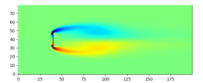
まとめ

雛形のコードを修正するだけですぐに実行できた。
格子ボルツマン法の理解はまだできていないので、ドキュメントを読んで別途投稿しようと思う。
速度空間という考え方がキーになると思われる。そのあたりの説明をしっかりしようと思う。