Google TrendのデータをAPI経由で取得し時系列解析〜人気プログラム言語のトレンドを考察する〜

Summary

• Google Trendから各キーワードの検索データを取得し、時系列データ分析を行います
• Pytrendsという（非公式の）ライブラリを用いてデータを取得します
• statsmodelsを活用して、時系列解析を行い、各キーワードの検索トレンドを分析します（季節成分分解・相関マトリックス）

分析ゴール

• 各プログラム言語のキーワード検索傾向や関係性を把握する

対象データ

• 対象言語を以下として、Google trendから抽出する
  • JavaScript
  • Ruby
  • Python
  • PHP
  • Java
  • SQL
• 2014年〜2018年9月末の期間で考察する

データ取得方法

• Pytrendsを利用して、Google Trend APIへアクセス
• 公式サイト
  • https://pypi.org/project/pytrends/
• 使い方（データ取得）
  • TrendReqで接続言語とタイムゾーンを指定して、API接続する
  • 検索キーワードをリストで渡す（キーワードが４つ以上だとエラーになります）
  • timeframeに期間をし、geoにエリア（国名を英２字）を指定する
    • 国名を英２字はCountry Abbreviationを参照
      • https://www.ncbi.nlm.nih.gov/books/NBK7249/
  • データはpandas.DataFrame形でリターンされる

from pytrends.request import TrendReq
# API Connection
pytrends = TrendReq(hl='ja-JP', tz=360)
# Set the search keyword
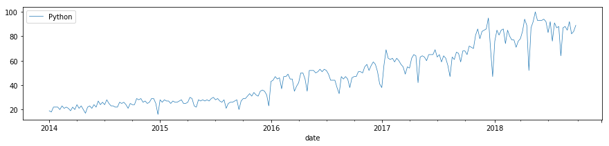
kw_list = ["Python"]
pytrends.build_payload(kw_list, timeframe='2014-01-01 2018-09-30', geo='JP')
df = pytrends.interest_over_time()
df.plot(figsize=(15, 3), lw=.7)

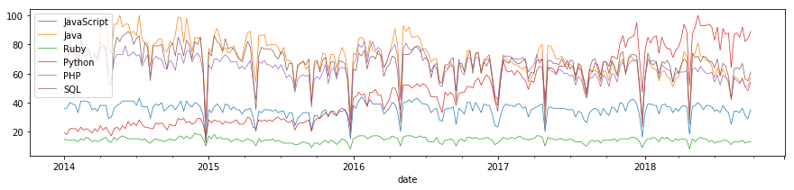
対象データの可視化

• 対象プログラム言語の文字列をリスト化して、prtrendに渡す
• 4ワード以上を投げるとエラーとなるので、2リストに分けてデータ出力した後、データフレームを結合する

kw_list1 = ["JavaScript","Java","Ruby"]
kw_list2 = ["Python", "PHP", "SQL"]

pytrends.build_payload(kw_list1, timeframe='2014-01-01 2018-09-30', geo='JP')
df1 = pytrends.interest_over_time()
pytrends.build_payload(kw_list2, timeframe='2014-01-01 2018-09-30', geo='JP')
df2 = pytrends.interest_over_time()
df = pd.concat([df1, df2], axis=1)
df.plot(figsize=(15, 3), lw=.7)

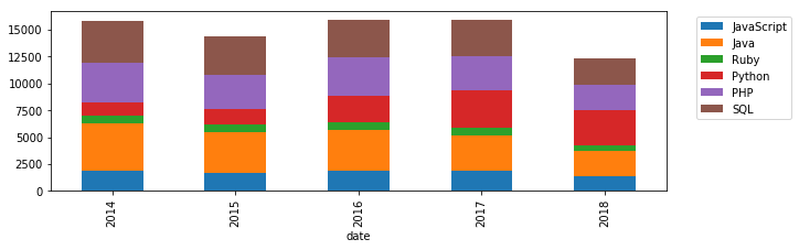
• 年次単位で集計して、合計アクセス数を算出する

yearly = df.resample('Y').sum().plot.bar(stacked=True, figsize=(10, 3))
plt.xticks(np.arange(5), ('2014', '2015', '2016', '2017', '2018'))
plt.legend(bbox_to_anchor=(1.04,1), loc="upper left")
plt.show()

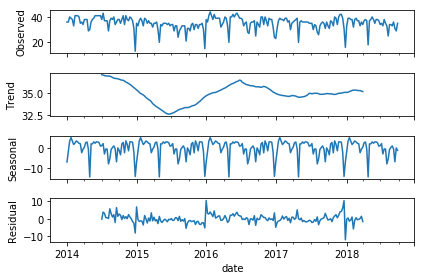
対象データ分析

• 季節性（年末や連休で減少）と周期性（年次周期）があるので、Seasonal decompositionを施して、トレンドを出力する
• Residualsのデータで時系列データの相関係数を出力し、各言語の検索状況の相関をみてみる
  • データ「JavaScript」で試してみる

res = sm.tsa.seasonal_decompose(df['JavaScript'])
res.plot()

• 全データに適用し、Trendのみ抽出して比較する

seasonality = pd.DataFrame()
for i in df.columns:
    res = sm.tsa.seasonal_decompose(df[i])
    seasonality = pd.concat([seasonality, res.trend], axis=1)

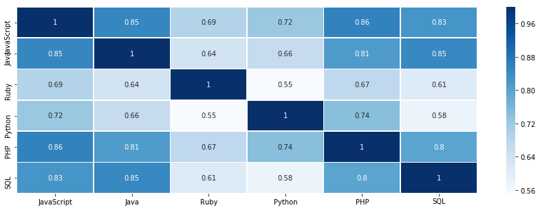
• 次に時系列データの相関係数を算出する
• 相関マトリックスを作成して、ヒートマップで可視化する

resid = pd.DataFrame()
for i in df.columns:
    res = sm.tsa.seasonal_decompose(df[i])
    resid = pd.concat([resid, res.resid], axis=1)
cor_matrix = resid.corr()

plt.figure(figsize=(15, 5))
sns.heatmap(cor_matrix, annot=True, lw=0.7, cmap='Blues')

分析結果の考察

• Pythonは長期にわたって上昇傾向、JavaScriptはほぼ一定の推移である
• Java, SQL, PHPはやや減少傾向にある
• 検索トレンドと人気ランキングとの相関があるかは不明
• "Google検索"そのものの検索数の変化（Google検索の普及率など）も加味して解釈が必要である

最後に

• データ分析が専門で、プログラミング言語についての知見は深くないので、何か観点があればフィードバック頂けますと幸いです
• 将来的にGoogle Trendの数値から何かを予測する取り組みができれば面白いと思いました
• エリア指定もできるので、国別のプログラミング言語の検索の違いなども次回挑戦してみようと思います