はじめに
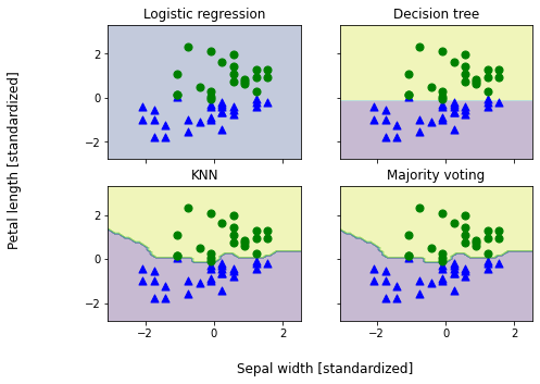
Python機械学習プログラミング 達人データサイエンティストによる理論と実践 の 7.3 アンサンブル分類器の評価とチューニング のサンプルプログラムを実行していて不思議な結果を得ました。下図のように、ロジスティック回帰による予測がうまくいってません。原因がよくわからなかったので調べることにしました。
因みにここでのお題は「Iris データを用いて、萼片の幅と花弁の長さから versicolor と versinica を分類する」というものになります。
結論
- train_test_split() 関数によって抽出された学習データに含まれる versicolor の個数と versinica の個数とが不一致だった
- 上記条件で、ロジスティック回帰のソルバーとして L-BFGS を用いていた
前提
| ソフトウエア | バージョン |
|---|---|
| Python | 3.10.0 |
| scikit-learn | 1.0.1 |
| scipy | 1.7.3 |
なお私が読んでいる「Python機械学習プログラミング 達人データサイエンティストによる理論と実践」は第一版となりますので、とても古い scikit-learn に基づいて書かれたものとなります。
問題の調査
使用したコード
まず上図を得るのに使用したコードは以下の通りです。
import numpy as np
import operator
import matplotlib.pyplot as plt
from itertools import product
from sklearn import datasets
from sklearn.preprocessing import StandardScaler
from sklearn.preprocessing import LabelEncoder
from sklearn.model_selection import train_test_split
from sklearn.linear_model import LogisticRegression
from sklearn.tree import DecisionTreeClassifier
from sklearn.neighbors import KNeighborsClassifier
from sklearn.pipeline import Pipeline
from sklearn.base import BaseEstimator
from sklearn.base import ClassifierMixin
from sklearn.base import clone
from sklearn.pipeline import _name_estimators


class MajorityVoteClassifier(BaseEstimator,
                             ClassifierMixin):
    """ A majority vote ensemble classifier

    Parameters
    ----------
    classifiers : array-like, shape = [n_classifiers]
      Different classifiers for the ensemble

    vote : str, {'classlabel', 'probability'} (default='classlabel')
      If 'classlabel' the prediction is based on the argmax of
        class labels. Else if 'probability', the argmax of
        the sum of probabilities is used to predict the class label
        (recommended for calibrated classifiers).

    weights : array-like, shape = [n_classifiers], optional (default=None)
      If a list of `int` or `float` values are provided, the classifiers
      are weighted by importance; Uses uniform weights if `weights=None`.

    """
    def __init__(self, classifiers, vote='classlabel', weights=None):

        self.classifiers = classifiers
        self.named_classifiers = {key: value for key, value
                                  in _name_estimators(classifiers)}
        self.vote = vote
        self.weights = weights

    def fit(self, X, y):
        """ Fit classifiers.

        Parameters
        ----------
        X : {array-like, sparse matrix}, shape = [n_examples, n_features]
            Matrix of training examples.

        y : array-like, shape = [n_examples]
            Vector of target class labels.

        Returns
        -------
        self : object

        """
        if self.vote not in ('probability', 'classlabel'):
            raise ValueError("vote must be 'probability' or 'classlabel'"
                             "; got (vote=%r)"
                             % self.vote)

        if self.weights and len(self.weights) != len(self.classifiers):
            raise ValueError('Number of classifiers and weights must be equal'
                             '; got %d weights, %d classifiers'
                             % (len(self.weights), len(self.classifiers)))

        # Use LabelEncoder to ensure class labels start with 0, which
        # is important for np.argmax call in self.predict
        self.lablenc_ = LabelEncoder()
        self.lablenc_.fit(y)
        self.classes_ = self.lablenc_.classes_
        self.classifiers_ = []
        for clf in self.classifiers:
            fitted_clf = clone(clf).fit(X, self.lablenc_.transform(y))
            self.classifiers_.append(fitted_clf)
        return self

    def predict(self, X):
        """ Predict class labels for X.

        Parameters
        ----------
        X : {array-like, sparse matrix}, shape = [n_examples, n_features]
            Matrix of training examples.

        Returns
        ----------
        maj_vote : array-like, shape = [n_examples]
            Predicted class labels.

        """
        if self.vote == 'probability':
            maj_vote = np.argmax(self.predict_proba(X), axis=1)
        else:  # 'classlabel' vote

            #  Collect results from clf.predict calls
            predictions = np.asarray([clf.predict(X)
                                      for clf in self.classifiers_]).T

            maj_vote = np.apply_along_axis(
                                      lambda x:
                                      np.argmax(np.bincount(x,
                                                weights=self.weights)),
                                      axis=1,
                                      arr=predictions)
        maj_vote = self.lablenc_.inverse_transform(maj_vote)
        return maj_vote

    def predict_proba(self, X):
        """ Predict class probabilities for X.

        Parameters
        ----------
        X : {array-like, sparse matrix}, shape = [n_examples, n_features]
            Training vectors, where n_examples is the number of examples and
            n_features is the number of features.

        Returns
        ----------
        avg_proba : array-like, shape = [n_examples, n_classes]
            Weighted average probability for each class per example.

        """
        probas = np.asarray([clf.predict_proba(X)
                             for clf in self.classifiers_])
        avg_proba = np.average(probas, axis=0, weights=self.weights)
        return avg_proba

    def get_params(self, deep=True):
        """ Get classifier parameter names for GridSearch"""
        if not deep:
            return super(MajorityVoteClassifier, self).get_params(deep=False)
        else:
            out = self.named_classifiers.copy()
            for name, step in self.named_classifiers.items():
                for key, value in step.get_params(deep=True).items():
                    out['%s__%s' % (name, key)] = value
            return out

iris = datasets.load_iris()
X, y = iris.data[50:, [1, 2]], iris.target[50:]
le = LabelEncoder()
y = le.fit_transform(y)

X_train, X_test, y_train, y_test = train_test_split(X, y, test_size=0.5, random_state=1)
sc = StandardScaler()
X_train_std = sc.fit_transform(X_train)

clf1 = LogisticRegression(penalty='l2',
                          C=0.001,
                          random_state=1)

clf2 = DecisionTreeClassifier(max_depth=1,
                              criterion='entropy',
                              random_state=0)

clf3 = KNeighborsClassifier(n_neighbors=1,
                            p=2,
                            metric='minkowski')

pipe1 = Pipeline([['sc', StandardScaler()],
                  ['clf', clf1]])
pipe3 = Pipeline([['sc', StandardScaler()],
                  ['clf', clf3]])

clf_labels = ['Logistic regression', 'Decision tree', 'KNN']

mv_clf = MajorityVoteClassifier(classifiers=[pipe1, clf2, pipe3])
clf_labels += ['Majority voting']
all_clf = [pipe1, clf2, pipe3, mv_clf]

x_min = X_train_std[:, 0].min() - 1
x_max = X_train_std[:, 0].max() + 1
y_min = X_train_std[:, 1].min() - 1
y_max = X_train_std[:, 1].max() + 1

xx, yy = np.meshgrid(np.arange(x_min, x_max, 0.1),
                     np.arange(y_min, y_max, 0.1))

f, axarr = plt.subplots(nrows=2, ncols=2,
                        sharex='col',
                        sharey='row',
                        figsize=(7, 5))

for idx, clf, tt in zip(product([0, 1], [0, 1]),
                        all_clf, clf_labels):
    clf.fit(X_train_std, y_train)

    Z = clf.predict(np.c_[xx.ravel(), yy.ravel()])
    Z = Z.reshape(xx.shape)

    axarr[idx[0], idx[1]].contourf(xx, yy, Z, alpha=0.3)

    axarr[idx[0], idx[1]].scatter(X_train_std[y_train==0, 0],
                                  X_train_std[y_train==0, 1],
                                  c='blue',
                                  marker='^',
                                  s=50)

    axarr[idx[0], idx[1]].scatter(X_train_std[y_train==1, 0],
                                  X_train_std[y_train==1, 1],
                                  c='green',
                                  marker='o',
                                  s=50)

    axarr[idx[0], idx[1]].set_title(tt)

plt.text(-3.5, -5.,
         s='Sepal width [standardized]',
         ha='center', va='center', fontsize=12)
plt.text(-12.5, 4.5,
         s='Petal length [standardized]',
         ha='center', va='center',
         fontsize=12, rotation=90)

plt.show()
scikit-learn のバージョン依存
先述の通り、参考にしている書籍はバージョン0.15.2に基づいています。scikit-learn のバージョンをいろいろ試した結果、期待される結果が得られるか否かは以下のようになりました。
| バージョン | 結果 |
|---|---|
| 0.19.2 | ○ |
| 0.20.4 | ○ |
| 0.21.3 | ○ |
| 0.22.2 | ☓ |
| 1.0.1 | ☓ |
0.22系の前後で大きく変わったことは、ロジスティック回帰のデフォルトのソルバーがliblinearからlbfgsになったことになります。試しにバージョン0.21.3を用いて、ソルバーとして明示的にlbfgsを指定したところ、上掲と同じ(ロジスティック回帰でうまく予測できていない)図が得られています。
L-BFGS法の損失関数
L-BFGS法では以下の損失関数を最小化することで重みパラメタ($\boldsymbol{w}$)を求めています。
l(\boldsymbol{w}) = \sum_{i=1}^n\log(1+e^{-y_i\boldsymbol{w}^{\mathrm{T}}\boldsymbol{x}_i}) + \frac{\alpha}{2}\boldsymbol{w}^{\mathrm{T}}\cdot\boldsymbol{w}
\tag{1}
ここで $n$ はデータ数、$\boldsymbol{x}$ は学習データ、$y$ はクラスラベル、$\alpha$ は正則化パラメタです。上述のコードでは $n=50$、$y\in \{-1,1\}$、$\alpha = 1/C = 1000$ となります。また
\boldsymbol{w}^{\mathrm{T}}\boldsymbol{x}_i = w_0 + w_1 x_i^{(1)} + w_2 x_i^{(2)}
\tag{2}
\boldsymbol{w}^{\mathrm{T}}\cdot\boldsymbol{w} = w_1^2 + w_2^2
\tag{3}
ここで $x_i^{(1)}$ は萼片の幅、$x_i^{(2)}$ は花弁の長さとなります。
さて、$\alpha \gg 1$ の場合には $\boldsymbol{w} \sim \boldsymbol{0}$ となりますので、$w_1 = w_2 = 0$ と仮定して、切片 $w_0$ の値によって $l(\boldsymbol{w})$ がどのように変化するか見てみることにしましょう。
import numpy as np
from sklearn.linear_model._logistic import _logistic_loss
from sklearn import datasets
from sklearn.preprocessing import LabelEncoder
from sklearn.model_selection import train_test_split
from sklearn.preprocessing import StandardScaler
import matplotlib.pyplot as plt


iris = datasets.load_iris()
X, y = iris.data[50:, [1, 2]], iris.target[50:]
le = LabelEncoder()
y = le.fit_transform(y)

X_train, X_test, y_train, y_test = train_test_split(X, y, test_size=0.5, random_state=1)
sc = StandardScaler()
X_train_std = sc.fit_transform(X_train)

mask_classes = np.array([-1, 1])
pos_class = np.array([1])
mask = y_train == pos_class
y_bin = np.ones(y_train.shape, dtype=X_train_std.dtype)
y_bin[~mask] = -1.0

target = y_bin

w0 = np.arange(-0.5, 0.52, 0.02)

loss = np.zeros_like(w0)
C = 0.001
loss = [_logistic_loss(np.array([0, 0, w0[i]]), X_train_std, target, alpha=1.0/C) for i in range(w0.size)]

plt.plot(w0, loss)
plt.xlabel('$w_0$')
plt.ylabel('loss function')
plt.show()
print(w0[np.argmin(loss)])
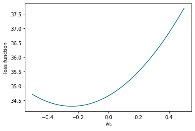
損失関数を最小にする切片の値は凡そ -0.24 であることがわかりました。試しにロジスティック回帰で求められた切片および重みパラメタの値は以下の通りです。
print(clf1.coef_[0], clf1.intercept_[0])
[0.00702671 0.01997023] -0.24119591913179658
この重みパラメタであれば、標準化された萼片の幅および花弁の長さの値が [-2, 2] の範囲では (2) 式から明らかなように全て負値となり、つまり全てが versicolor に分類されてしまいます。
なぜ $w_0$ が有意な値($|w_0| \gg 0$)を持ってしまうのでしょうか?それは (1) 式の対数項を以下のように分離するとわかりやすくなります。
\begin{array}{rcl}
\displaystyle{\sum_{i=1}^n\log(1+e^{-y_i\boldsymbol{w}^{\mathrm{T}}\boldsymbol{x}_i})} & = & \displaystyle{\sum_{i:y_i=1}\log(1+e^{-\boldsymbol{w}^{\mathrm{T}}\boldsymbol{x}_i})} + \displaystyle{\sum_{i:y_i=-1}\log(1+e^{\boldsymbol{w}^{\mathrm{T}}\boldsymbol{x}_i})} \\
& \sim & n_1\log(1+e^{-w_0}) + n_{-1}\log(1+e^{w_0})
\end{array}
ここで $n_1$ は $y_i=1$ となるデータ数、$n_{-1}$ は $y_i=-1$ となるデータ数です。この関数は第一項が単調減少、第二項が単調増加関数となります。したがって $n_1=n_{-1}$ であれば $w_0=0$ の時に極小値を与えます。たとえば $n_1<n_{-1}$ の場合には極小値が左にずれます。
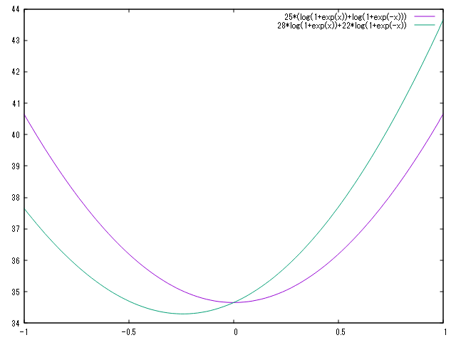
つまり学習データにおいて versicolor と versinica のデータ数が一致していないことが示唆されます。確認してみると確かにそのとおりでした。
print(np.sum(y_train==1),np.sum(y_train==0))
22 28
コードの修正
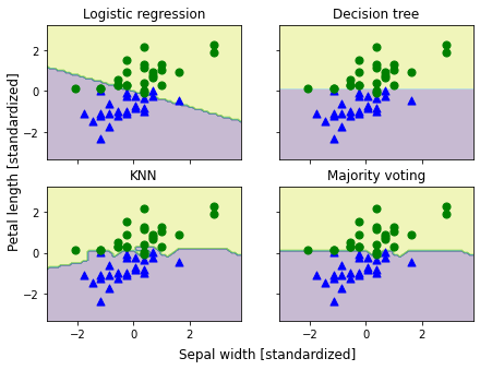
第三版に掲載されているコードは github で公開されており、それによれば学習データとテストデータの分離をするために引数として stratify が指定されていました。すなわち、
X_train, X_test, y_train, y_test = train_test_split(X, y, test_size=0.5, random_state=1, stratify=y)
これによって 25 個ずつ抽出されるようになり、この学習データを用いることによって、以下のような期待される結果を得ることができました。
まとめ
L-BFGS法を用いてロジスティック回帰で二値分類するにあたり、正則化パラメタが極めて大きい場合には、学習データとして各クラスのデータ数を同じにする必要があります。