ベータ分布を使ったベルヌーイ分布のパラメータ学習（MLSベイズ図3.3）

目的

• 機械学習スタートアップシリーズ「ベイズ推論による機械学習入門」の図をJuliaで再現する
• 今回の対象: 図3.3 ベータ分布を使ったベルヌーイ分布のパラメータ学習

ベータ分布、ベルヌーイ分布の計算

• Distributions.jlから利用できる

using Distributions
μtruth = 0.25
dist = Bernoulli(μtruth)
println(rand(dist, 10))

# ==> [0, 0, 1, 1, 1, 0, 0, 0, 0, 1]  (コインを10回ふった結果）

ベータ分布のプロット

• IJuliaをインストールして、Jupyter Notebook上で実行する
• 描画はPlots.jlを使い、バックエンドはGR Frameworkとする
• 0付近と1付近が危ないので少し避けておく

using Plots
gr()

ϵ = 0.01;
x = linspace(ϵ, 1.0 - ϵ, N);
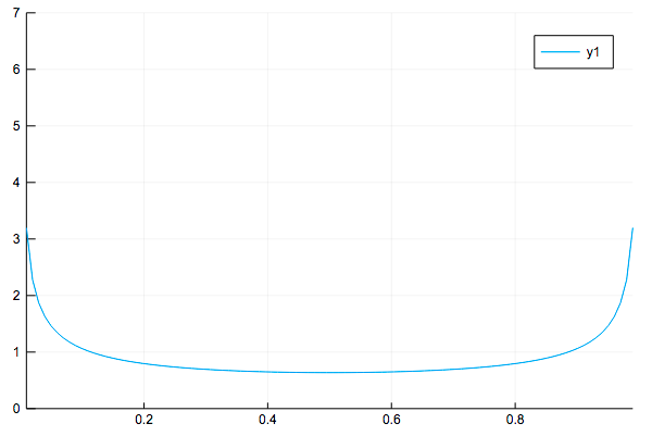
bdist = Beta(0.5, 0.5)
y = pdf.(bdist, x)
plot(x, y, ylim=(0.0, 7.0))

• プロットの例

学習

• コインをふって表の出た回数と裏の出た回数（総数 - 表の出た回数）を計数し、ベータ分布のパラメータα、βに加算して更新する（詳しくは本などを参照）
• サンプル数は$N=50$まで

• $\alpha, \beta$の初期値は適当に決めて良い

  • 本と同じく、$N=1, 3, 10, 50$のときだけ結果をプロットする

• パラメータ更新部分

nsample = 50;
α = 10.
β = 5.
bdist = Beta(α, β)
d1 = (α, β)
samples = Int64[]
lα = [α]
lβ = [β]
for i in 1:nsample
    ni = rand(dist)
    push!(samples, ni)  # サンプル

    pos = sum(samples)  # 1の回数
    neg = i - pos       # 総数 - 1の回数
    push!(lα, α + pos)
    push!(lβ, β + neg)
end
pos = sum(samples)
neg = nsample - pos
push!(lα, α + pos)
push!(lβ, β + neg)
println(samples)
println(lα, lβ)

• プロット部

ldist = []
indices = [1, 3, 10, 50]
for idx in indices
    αi = lα[idx]
    βi = lβ[idx]
    disti = Beta(αi, βi)
    push!(ldist, disti)
end

# beta dist plot
plot()
for i in 1:4
    yi = pdf.(ldist[i], x);
    plot!(x, yi, ylim=(0.0, 7.0))
end
plot!()

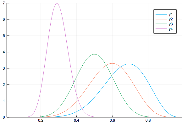
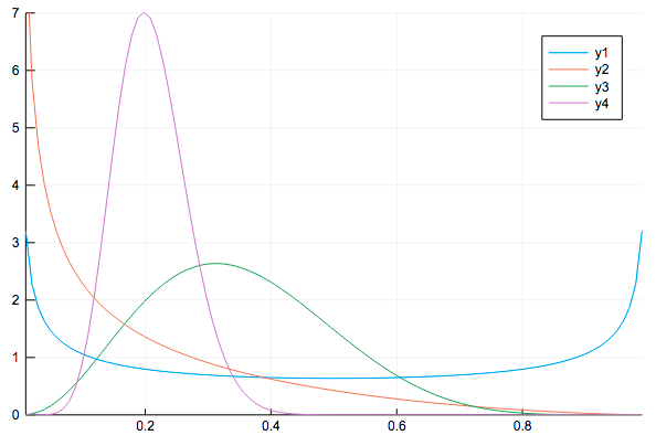
• 本を真似して$(0.5, 0.5)$、$(1., 1.)$、$(10., 5.)$を初期値として、結果を確認する

• $(0.5, 0.5)$からスタートする場合

• $(1., 1.)$からスタートする場合

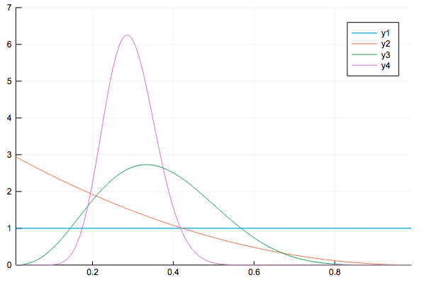
• $(10., 5.)$からスタートする場合