はじめに
前回の記事では最初の一歩を解説したが、より細かな使い方についても述べる
トラジェクトリーの読み込みとトポロジーの取得
今後の記載は以下を行っているものとして進めます。
import mdtraj as md
t = md.load('md.xtc', top='md.gro')
top = t.topology
原子・残基の選択など
残基数、原子数
# 原子数
print(t.n_atoms)
# 残基数
print(t.n_residues)
i番目の原子
こちらも0始まり。
top.atom(i)
すべての残基の名前を出力する
#t.n_residuesで残基数
for i in range(t.n_residues):
    print(top.residue(i).name)
○番目の残基に含まれる全原子のインデックスを得る
ただし、residは0始まりなことに注意
#10番目から30番目までの残基を選択
atom_list = top.select("resid 10 to 30")
#同義
atom_list = top.select("(10 <= resid) and (resid <= 30)")
特定のアミノ酸のみのインデックスを得る
#LYSのみのインデックスを得る
atom_list = top.select('resname LYS')
i番目の残基に含まれる全原子のインデックスを得る
ただし、residは0始まりなことに注意
atom_list = top.select('resid '+str(i))
水素以外のインデックスを得る
atom_list = top.select("symbol != H")
CA原子のみのインデックスを得る
atom_list = top.select("name CA")
proteinのみ、backboneのみ、sidechainのみのインデックスを得る
#proteinのみ
atom_list = top.select("is_protein True")
#backboneのみ
atom_list = top.select("is_backbone True")
#sidechainのみ
atom_list = top.select("is_sidechain True")
○番目の原子のインデックスを得る
原子の番号はindexで指定できる。
indexは0始まりであることに注意
#10番目から30番目までの原子を選択(21原子が選択される)
atom_list = top.select("index 10 to 30")
○番目のChainに含まれる原子のインデックスを得る
chainidで指定できる。これも0始まり。
#1番目のchainを選択
atom_list = top.select("chainid 1")
トラジェクトリーから指定する原子の分だけ取り出す
t_slice = t.atom_slice(atom_list)
トポロジーをpandasのデータフレームに変換する
atoms, bonds = top.to_dataframe()
atoms

bonds

これをやるメリットですが、例えば、特定の残基を削除したり、ChainIDを変更することがやりやすいです。
公式の例ですと、二面角を計算する際に、原子のインデックスを確認する目的で使用されています。
ここではデータフレームを編集して残基名を変更した後に再びトポロジーに戻しましょう。
atoms = atoms.replace(
  {
    "resName":{'MET':'AAA'}
  }
)
METがAAAに変わったことがわかります。

あとはデータフレームをトポロジーに変換します。
top2 = md.Topology.from_dataframe(atoms, bonds)
構造のアライメントを行う
#トラジェクトリtのフレーム0を参照構造として、atom_listの原子を使って向きを揃える
t = t.superpose(t, frame=0, atom_indices=atom_list)
#フレーム0を使い、位置合わせにすべての原子を使う場合は以下でも良い
t = t.superpose(t)
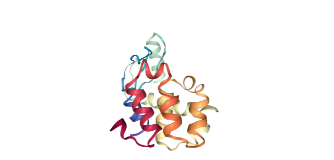
構造の可視化
MDTraj単体では可視化できませんが、nglviewを使うと可視化できます。
まずはインストール。
conda install nglview -c conda-forge
以下のコマンドで実行です。
import mdtraj as md
import nglview as nv

traj = md.load('./md.xtc', top='md.gro')

view = nv.show_mdtraj(traj)
view
Jupyterノートブック上で動画再生できます。
MD結果の解析
RMSDを計算する
rmsds = md.rmsd(t, t, 0)

2つ目の引数で参照構造としてtを使うこと、3つ目の引数で参照構造の0フレーム目を使うことを指定している。
CA原子のみのRMSDを計算したければ、以下のようにする。
atom_list = top.select("name CA")
rmsds = md.rmsd(t, t, 0, atom_indices=atom_list)
グラフ描画してみてもよいでしょう。
import matplotlib.pyplot as plt

plt.plot(t.time, rmsds, label="rmsd")
plt.xlabel('time [ps]')
plt.ylabel('rmsd [nm]')
plt.show()
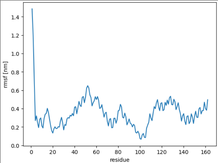
RMSFを計算する
atom_list = top.select("name CA")
rmsfs = md.rmsf(t, t, 0, atom_indices=atom_list)
RMSFは「平均構造からの揺らぎ」なので、フレーム数を指定するのは違う気がしますが、これがないと動きません。マニュアルの記載もちょっと変。誰かわかったら教えてください。
import matplotlib.pyplot as plt

#残基IDのリストを作成する
resid_list = []
for a in atom_list:
    resid_list.append(top.atom(a).residue.index+1)

#描画
plt.plot(resid_list, rmsfs, label="rmsd")
plt.xlabel('residue')
plt.ylabel('rmsf [nm]')
plt.show()
PCAを行う
座標に対してPCA解析を行いましょう。
from __future__ import print_function
%matplotlib inline
import mdtraj as md
import matplotlib.pyplot as plt
from sklearn.decomposition import PCA

pca1 = PCA(n_components=2)
t.superpose(t, 0)

reduced_cartesian = pca1.fit_transform(t.xyz.reshape(t.n_frames, t.n_atoms * 3))
print(reduced_cartesian.shape)

plt.figure()
plt.scatter(reduced_cartesian[:, 0], reduced_cartesian[:,1], marker='x', c=t.time)
plt.xlabel('PC1')
plt.ylabel('PC2')
plt.title('Cartesian coordinate PCA')
cbar = plt.colorbar()
cbar.set_label('Time [ps]')

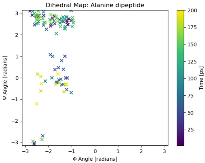
二面角を計算する
公式の例からそのまま記載します。
ψとΦを計算するためにそれぞれ二面角を構成する原子のインデックスを含むリストを作成します。
あとはconpute_dihedralsにトラジェクトリと原子のインデックスを渡すだけです。
psi_indices, phi_indices = [6, 8, 14, 16], [4, 6, 8, 14]
angles = md.compute_dihedrals(t, [phi_indices, psi_indices])
anglesに各フレームのψとΦが格納されます。
ラマチャンドランプロットを描画してみましょう。
%matplotlib inline
from pylab import *
from math import pi

figure()
title('Dihedral Map: Alanine dipeptide')
scatter(angles[:, 0], angles[:, 1], marker='x', c=t.time)
cbar = colorbar()
cbar.set_label('Time [ps]')
xlabel(r'$\Phi$ Angle [radians]')
xlim(-pi, pi)
ylabel(r'$\Psi$ Angle [radians]')
ylim(-pi, pi)
距離を計算する
原子ペア(1,2),(3,4),(5,6),(7,8)それぞれについて、最初の5フレームにおける距離を計算する
pair_list = np.array([[1,2],[3,4],[5,6],[7,8]])
distance = md.compute_distances(t[:5],pair_list)
print(distance)
#結果は↓
[[0.15976545 0.205565   0.2156988  0.17370385]
 [0.1643501  0.20190595 0.21467426 0.18251847]
 [0.15955558 0.21631935 0.22040404 0.18016115]
 [0.15979047 0.21072258 0.21478376 0.17570712]
 [0.1536686  0.21158913 0.20508307 0.18028308]]
重心を計算する
最初の5フレームのトラジェクトリー全体の重心を計算する
com = md.compute_center_of_mass(t[:5])
print(com)

#結果は↓ 重心座標のxyz
[[3.45930822 3.48708447 3.47640435]
 [3.45666188 3.48816336 3.47538709]
 [3.45537152 3.49009828 3.47515898]
 [3.45710578 3.48709138 3.47764402]
 [3.4582961  3.48730801 3.47942968]]
もちろんスライスすれば特定原子集団の重心を求めることも可能
0番目の残基の重心座標を最初の5フレーム分出力するには
atom_list = top.select('resid '+str(0))
t_slice = t.atom_slice(atom_list)

com = md.compute_center_of_mass(t_slice[:5])
print(com)

#結果は↓ 重心座標のxyz
[[4.38645248 3.06147587 2.47268419]
 [4.42610573 3.07630685 2.41688386]
 [4.42688007 3.09259641 2.47004827]
 [4.51419426 3.11977723 2.48547242]
 [4.49403277 3.09523345 2.49413727]]
トラジェクトリの操作
トラジェクトリの保存
#トラジェクトリをxtcファイルで保存
t.save_xtc('md-01.xtc')
xtc以外にもdcdやpdbなど様々なフォーマットがサポートされています。
詳しくは下記ページを確認してください。
トラジェクトリの結合(原子)
#トラジェクトリからproteinのみスライス
atom_list = top.select('is_protein True')
t_slice_protein = t.atom_slice(atom_list)
#waterのみスライス
atom_list = top.select('is_water True')
t_slice_water = t.atom_slice(atom_list)
#proteinとwaterのトラジェクトリを合体
t_slice_stack = t_slice_protein.stack(t_slice_water)
トラジェクトリの結合(時間)
#1-10フレーム目をスライス
t_slice_0_10 = t[0:10]
#11-20フレーム目をスライス
t_slice_10_20 = t[10:20]
#2つのトラジェクトリを結合(1-20フレームのトラジェクトリを生成)
t_join = t_slice_0_10.join(t_slice_10_20)
ユニットセルの長さ
#各フレームにおけるユニットセルの長さ
print(t.unitcell_lengths)
#結果は↓
[[6.9481483 6.9481483 6.9481483]
 [6.9548845 6.9548845 6.9548845]
 [6.948615  6.948615  6.948615 ]
 [6.959194  6.959194  6.959194 ]
 [6.9590874 6.9590874 6.9590874]
・・・
 [6.966455  6.966455  6.966455 ]]

#最終フレームにおけるユニットセルの長さ
print(t.unitcell_lengths[-1])
#結果は↓
[6.966455 6.966455 6.966455]
参考