この記事では以下のチュートリアルを参考に粗視化力場「Martini」でタンパク質の計算を行う。
以下の流れでセットアップを行う。
-
原子レベルのタンパク質構造を粗視化モデルに変換する。
-
適切なMartiniトポロジーを生成する。
-
目的の環境下でタンパク質を溶媒和する。
ステップ1および2はmartinize.pyを用いて行う。
ステップ3はGROMACSのツールやその他のツールで行う。
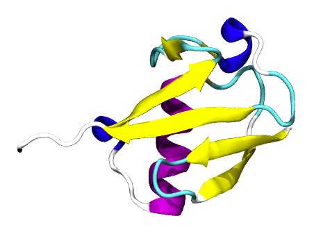
このチュートリアルではユビキチンのシミュレーションをセットアップする。
準備
martinize.pyをダウンロード
$ wget http://cgmartini.nl/images/stories/tutorial/2017/protein-tutorial-v2016.3/soluble-protein/ubiquitin/martini/martinize.py
worked fileをダウンロード
必要ではない。作業の確認に。
$ wget http://cgmartini.nl/images/stories/tutorial/2017/protein-tutorial-v2016.3/soluble-protein/ubiquitin.tgz
ユビキチンのPDBファイルをダウンロードする
$ wget http://www.rcsb.org/pdb/files/1UBQ.pdb.gz
$ gunzip 1UBQ.pdb.gz
DSSPのインストール
自分はUbuntuの環境なので下記コマンドでインストールした。
「dssp」コマンドが使えるようになればOK
sudo apt install dssp
python環境の準備
また、martinize.pyはpythonのバージョンが2.6もしくは2.7である必要があるため、condaなどでpython環境を整えておく。
conda activate py27
Martiniトポロジーの作成
martinize.pyを実行してユビキチンのトポロジーを生成する。
dsspコマンドのパスは各々の環境に合わせて変える。
$ python martinize.py -f 1UBQ.pdb -o single-ubq.top -x 1UBQ-CG.pdb -dssp /usr/bin/dssp -p backbone -ff martini22

INFO       MARTINIZE, script version 2.6
INFO       If you use this script please cite:
INFO       de Jong et al., J. Chem. Theory Comput., 2013, DOI:10.1021/ct300646g
INFO       Chain termini will be charged
INFO       Residues at chain brakes will not be charged
INFO       The martini22 forcefield will be used.
INFO       Local elastic bonds will be used for extended regions.
INFO       Position restraints will be generated.
WARNING    Position restraints are only enabled if -DPOSRES is set in the MDP file
INFO       Read input structure from file.
INFO       Input structure is a PDB file.
INFO       Found 2 chains:
INFO          1:   A (Protein), 602 atoms in 76 residues.
INFO          2:   A (Water), 58 atoms in 58 residues.
INFO       Removing 58 water molecules (chain A).
INFO       Total size of the system: 76 residues.
INFO       Writing coarse grained structure.
INFO       (Average) Secondary structure has been determined (see head of .itp-file).
INFO       Created coarsegrained topology
INFO       Written 1 ITP file
INFO       Output contains 1 molecules:
INFO          1->  Protein_A (chain  A)
INFO       Written topology files
INFO       Note: Cysteine bonds are 0.24 nm constraints, instead of the published 0.39nm/5000kJ/mol.

	There you are. One MARTINI. Shaken, not stirred.


The chromatic scale is what you use to give the effect of drinking a quinine martini and having an enema simultaneously.
                                                                 --Philip Larkin
このコマンドでmartini力場のバージョン2.2を指定している。二次構造の指定にDSSPを使ったが、二次構造のファイル*.ssdで指定することも可能である。その場合は以下のようにする。
$ python martinize.py -f 1UBQ.pdb -o single-ubq.top -x 1UBQ-CG.pdb -ss <YOUR FILE> -p backbone -ff martini22
なお、martinize.pyの説明は
$ python martinize.py -h
で見ることができる。
新しいファイル、
chain_A.ssd
single-ubq.top
Protein_A.itp
1UBQ-CG.pdb
が生成された。
"chain_A.ssd"はDSSPにより特定された二次構造、"single-ubq.top"はトポロジーファイル、"Protein_A.itp"はユビキチンのトポロジーを示したファイル、"1UBQ-CG.pdb"は粗視化されたPDBファイルである。
Martiniトポロジーファイルの取得
よりmartini_v2.2.itp(先程指定した力場のバージョンと対応している)をダウンロードする。
ここに原子タイプの定義や、非結合相互作用のパラメータが記述されている。
MDPファイルの取得
より、martini_v2.x_new-rf.mdpをダウンロードする。
トポロジーファイルの変更
.topファイルの1行目を変更し、martiniの力場ファイルを読み込ませる
#include "martini_v2.2.itp"
ユビキチンをボックスにつめる
GROMACSのeditconfでユビキチンをボックスに詰める
gmx editconf -f 1UBQ-CG.pdb -d 1.0 -bt dodecahedron -o 1UBQ-CG.gro
エネルギー最小化計算の実行
ここで一度エネルギー最小化計算を行う
下記のようにMDPファイルを編集し、minimization.mdpとする。
title                    = Martini

; TIMESTEP IN MARTINI
; Most simulations are numerically stable with dt=40 fs,
; however better energy conservation is achieved using a
; 20-30 fs timestep.
; Time steps smaller than 20 fs are not required unless specifically stated in the itp file.

integrator               = steep
dt                       = 0.03
nsteps                   = 100
nstcomm                  = 100
comm-grps                        =

nstxout                  = 0
nstvout                  = 0
nstfout                  = 0
nstlog                   = 1000
nstenergy                = 100
nstxout-compressed       = 1000
compressed-x-precision   = 100
compressed-x-grps        =
energygrps               =

cutoff-scheme            = Verlet
nstlist                  = 20
ns_type                  = grid
pbc                      = xyz
verlet-buffer-tolerance  = 0.005

coulombtype              = reaction-field
rcoulomb                 = 1.1
epsilon_r                = 15   ; 2.5 (with polarizable water)
epsilon_rf               = 0
vdw_type                 = cutoff
vdw-modifier             = Potential-shift-verlet
rvdw                     = 1.1
下記コマンドでtprファイルの生成およびジョブの実行を行う。
$ gmx grompp -p single-ubq.top -f minimization.mdp -c 1UBQ-CG.gro -o minimization-vac.tpr
$ gmx mdrun -deffnm minimization-vac -v
溶媒を配置する
よりwater.groを取得し、下記コマンドで溶媒和する。
$ gmx solvate -cp minimization-vac.gro -cs water.gro -radius 0.21 -o solvated.gro
Generating solvent configuration
Will generate new solvent configuration of 2x2x2 boxes
Solvent box contains 1926 atoms in 1926 residues
Removed 643 solvent atoms due to solvent-solvent overlap
Removed 117 solvent atoms due to solute-solvent overlap
Sorting configuration
Found 1 molecule type:
      W (   1 atoms):  1166 residues
Generated solvent containing 1166 atoms in 1166 residues
Writing generated configuration to solvated.gro

Output configuration contains 1329 atoms in 1242 residues
Volume                 :     170.528 (nm^3)
Density                :      2122.5 (g/l)
Number of solvent molecules:   1166
ユビキチンのみのトポロジーを、全システムのトポロジーにするためファイル名を変更する。
cp single-ubq.top system.top
先程追加した水分子の分を追記する。
[ molecules ]
; name        number
Protein_A        1
W           1166
エネルギー最小化を実行
この状態で再びエネルギー最小化計算、平衡化計算、production runを実施する。
equilibration.mdpは
;
; STANDARD MD INPUT OPTIONS FOR MARTINI 2.x
; Updated 15 Jul 2015 by DdJ
;
; for use with GROMACS 5
; For a thorough comparison of different mdp options in combination with the Mar
tini force field, see:
; D.H. de Jong et al., Martini straight: boosting performance using a shorter cu
toff and GPUs, submitted.

title                    = Martini

; TIMESTEP IN MARTINI
; Most simulations are numerically stable with dt=40 fs,
; however better energy conservation is achieved using a
; 20-30 fs timestep.
; Time steps smaller than 20 fs are not required unless specifically stated in t
he itp file.

integrator               = md
dt                       = 0.02
nsteps                   = 10000
nstcomm                  = 100
comm-grps                        =

nstxout                  = 0
nstvout                  = 0
nstfout                  = 0
nstlog                   = 1000
nstenergy                = 100
nstxout-compressed       = 1000
compressed-x-precision   = 100
compressed-x-grps        =
energygrps               =
; NEIGHBOURLIST and MARTINI
; To achieve faster simulations in combination with the Verlet-neighborlist
; scheme, Martini can be simulated with a straight cutoff. In order to
; do so, the cutoff distance is reduced 1.1 nm.
; Neighborlist length should be optimized depending on your hardware setup:
; updating ever 20 steps should be fine for classic systems, while updating
; every 30-40 steps might be better for GPU based systems.
; The Verlet neighborlist scheme will automatically choose a proper neighborlist
; length, based on a energy drift tolerance.
;
; Coulomb interactions can alternatively be treated using a reaction-field,
; giving slightly better properties.
; Please realize that electrostVatic interactions in the Martini model are
; not considered to be very accurate to begin with, especially as the
; screening in the system is set to be uniform across the system with
; a screening constant of 15. When using PME, please make sure your
; system properties are still reasonable.
;
; With the polarizable water model, the relative electrostatic screening
; (epsilon_r) should have a value of 2.5, representative of a low-dielectric
; apolar solvent. The polarizable water itself will perform the explicit screening
; in aqueous environment. In this case, the use of PME is more realistic.


cutoff-scheme            = Verlet
nstlist                  = 20
ns_type                  = grid
pbc                      = xyz
verlet-buffer-tolerance  = 0.005

coulombtype              = reaction-field
rcoulomb                 = 1.1
epsilon_r                = 15   ; 2.5 (with polarizable water)
epsilon_rf               = 0
vdw_type                 = cutoff
vdw-modifier             = Potential-shift-verlet
rvdw                     = 1.1
; MARTINI and TEMPERATURE/PRESSURE
; normal temperature and pressure coupling schemes can be used.
; It is recommended to couple individual groups in your system separately.
; Good temperature control can be achieved with the velocity rescale (V-rescale)
; thermostat using a coupling constant of the order of 1 ps. Even better
; temperature control can be achieved by reducing the temperature coupling
; constant to 0.1 ps, although with such tight coupling (approaching
; the time step) one can no longer speak of a weak-coupling scheme.
; We therefore recommend a coupling time constant of at least 0.5 ps.
; The Berendsen thermostat is less suited since it does not give
; a well described thermodynamic ensemble.
;
; Pressure can be controlled with the Parrinello-Rahman barostat,
; with a coupling constant in the range 4-8 ps and typical compressibility
; in the order of 10e-4 - 10e-5 bar-1. Note that, for equilibration purposes,
; the Berendsen barostat probably gives better results, as the Parrinello-
; Rahman is prone to oscillating behaviour. For bilayer systems the pressure
; coupling should be done semiisotropic.

tcoupl                   = berendsen ; v-rescale
tc-grps                  = system
tau_t                    = 2.0
ref_t                    = 300
Pcoupl                   = berendsen ; parrinello-rahman
Pcoupltype               = isotropic
tau_p                    = 12.0 ; 12.0  ;parrinello-rahman is more stable with larger tau-p, DdJ, 20130422
compressibility          = 3e-4 ;  3e-4
ref_p                    = 1.0  ; 1.0

gen_vel                  = yes
gen_temp                 = 300
gen_seed                 = 473529

; MARTINI and CONSTRAINTS
; for ring systems and stiff bonds constraints are defined
; which are best handled using Lincs.

constraints              = none
constraint_algorithm     = Lincs
また、dynamic.mdpは
;
; STANDARD MD INPUT OPTIONS FOR MARTINI 2.x
; Updated 15 Jul 2015 by DdJ
;
; for use with GROMACS 5
; For a thorough comparison of different mdp options in combination with the Martini force field, see:
; D.H. de Jong et al., Martini straight: boosting performance using a shorter cutoff and GPUs, submitted.

title                    = Martini

; TIMESTEP IN MARTINI
; Most simulations are numerically stable with dt=40 fs,
; however better energy conservation is achieved using a
; 20-30 fs timestep.
; Time steps smaller than 20 fs are not required unless specifically stated in the itp file.

integrator               = md
dt                       = 0.03
nsteps                   = 3000000
nstcomm                  = 100
comm-grps                        =

nstxout                  = 0
nstvout                  = 0
nstfout                  = 0
nstlog                   = 100000
nstenergy                = 100
nstxout-compressed       = 5000
compressed-x-precision   = 100
compressed-x-grps        =
energygrps               =
; NEIGHBOURLIST and MARTINI
; To achieve faster simulations in combination with the Verlet-neighborlist
; scheme, Martini can be simulated with a straight cutoff. In order to
; do so, the cutoff distance is reduced 1.1 nm.
; Neighborlist length should be optimized depending on your hardware setup:
; updating ever 20 steps should be fine for classic systems, while updating
; every 30-40 steps might be better for GPU based systems.
; The Verlet neighborlist scheme will automatically choose a proper neighborlist
; length, based on a energy drift tolerance.
;
; Coulomb interactions can alternatively be treated using a reaction-field,
; giving slightly better properties.
; Please realize that electrostVatic interactions in the Martini model are
; not considered to be very accurate to begin with, especially as the
; screening in the system is set to be uniform across the system with
; a screening constant of 15. When using PME, please make sure your
; system properties are still reasonable.
;
; With the polarizable water model, the relative electrostatic screening
; (epsilon_r) should have a value of 2.5, representative of a low-dielectric
; apolar solvent. The polarizable water itself will perform the explicit screening
; in aqueous environment. In this case, the use of PME is more realistic.


cutoff-scheme            = Verlet
nstlist                  = 20
ns_type                  = grid
pbc                      = xyz
verlet-buffer-tolerance  = 0.005

coulombtype              = reaction-field
rcoulomb                 = 1.1
epsilon_r                = 15   ; 2.5 (with polarizable water)
epsilon_rf               = 0
vdw_type                 = cutoff
vdw-modifier             = Potential-shift-verlet
rvdw                     = 1.1

; MARTINI and TEMPERATURE/PRESSURE
; normal temperature and pressure coupling schemes can be used.
; It is recommended to couple individual groups in your system separately.
; Good temperature control can be achieved with the velocity rescale (V-rescale)
; thermostat using a coupling constant of the order of 1 ps. Even better
; temperature control can be achieved by reducing the temperature coupling
; constant to 0.1 ps, although with such tight coupling (approaching
; the time step) one can no longer speak of a weak-coupling scheme.
; We therefore recommend a coupling time constant of at least 0.5 ps.
; The Berendsen thermostat is less suited since it does not give
; a well described thermodynamic ensemble.
;
; Pressure can be controlled with the Parrinello-Rahman barostat,
; with a coupling constant in the range 4-8 ps and typical compressibility
; in the order of 10e-4 - 10e-5 bar-1. Note that, for equilibration purposes,
; the Berendsen barostat probably gives better results, as the Parrinello-
; Rahman is prone to oscillating behaviour. For bilayer systems the pressure
; coupling should be done semiisotropic.

tcoupl                   = v-rescale
tc-grps                  = system
tau_t                    = 1.0
ref_t                    = 300
Pcoupl                   = parrinello-rahman
Pcoupltype               = isotropic
tau_p                    = 12.0 ; 12.0  ;parrinello-rahman is more stable with larger tau-p, DdJ, 20130422
compressibility          = 3e-4 ;  3e-4
ref_p                    = 1.0  ; 1.0

gen_vel                  = yes
gen_temp                 = 300
gen_seed                 = 473529

; MARTINI and CONSTRAINTS
; for ring systems and stiff bonds constraints are defined
; which are best handled using Lincs.

constraints              = none
constraint_algorithm     = Lincs
とする。
下記コマンドでジョブを実行する。
$ gmx grompp -p system.top -c solvated.gro -f minimization.mdp -o minimization.tpr
$ gmx mdrun -deffnm minimization -v
$ gmx grompp -p system.top -c minimization.gro -f equilibration.mdp -o equilibration.tpr
$ gmx mdrun -deffnm equilibration -v
$ gmx grompp -p system.top -c equilibration.gro -f dynamic.mdp -o dynamic.tpr -maxwarn 1
$ gmx mdrun -deffnm dynamic -v
以上でタンパク質のMDは終了。
計算時間は
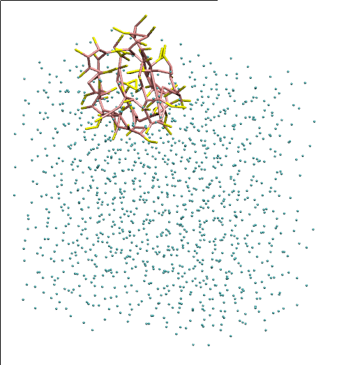
VMDによる可視化
まずトラジェクトリを変換して回転・並進の影響を除去する。
その後、VMDでトラジェクトリを開く。
$ gmx trjconv -f dynamic.xtc -s dynamic.tpr -fit rot+trans -o viz.xtc
$ vmd equilibration.gro viz.xtc
チュートリアルのページにある「cg_bonds-v5.tcl」をダウンロードし、VMDのtclコンソールで
source cg_bonds-v5.tcl
cg_bonds -top system.top
を実行することで結合情報を含めて可視化される。
ただし、二次構造は可視化されない。(何か方法があるのだろうか。せっかくなのだから二次構造も含めて見てみたい)
この後チュートリアルでは弾性ネットワークモデルを適用して、より高次構造を保つ試みを紹介している。
これもいつかやりたい。