In this section, we will cover the basics of geopandas, a Python library to interact with geospatial vector data.
Geopandas provides an easy-to-use interface to vector data sets. It combines the capabilities of pandas, the data analysis package we got to know in the Geo-Python course, with the geometry handling functionality of shapely, the geo-spatial file format support of fiona and the map projection libraries of pyproj.
geopandasによるベクターデータな基本的な処理をやっていきましょう。
geopandasは、pandasにshapely・fiona・pyproj(これは別途)などを組み込んだものです。
There is one key difference between pandas’s data frames and geopandas’ GeoDataFrames: a GeoDataFrame contains an additional column for geometries. By default, the name of this column is geometry, and it is a GeoSeries that contains the geometries (points, lines, polygons, …) as shapely.geometry objects.
pandasとの違いは、GeoDataFramesであること。GeoDataFramesは、GeoSeriesという型で、shapely.geometryオブジェクトを格納します。
まずは開始する前のお約束として、geopandasをインストールします。
! pip install geopandas
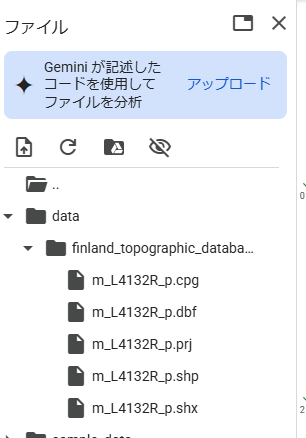
次に、読み込むファイル(m_L4132R_p.shp)をアップロードします。
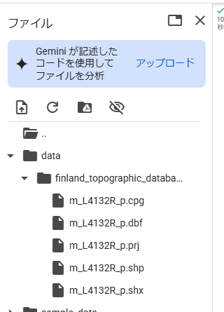
ファイルは https://github.com/mopinfish/auto-gis-notebooks/tree/main/lessons/lesson-2/data/finland_topographic_database にあります。
import pathlib
import geopandas
import numpy
import pandas

DATA_DIRECTORY = pathlib.Path().resolve() / "data"
print (DATA_DIRECTORY)
HIGHLIGHT_STYLE = "background: #f66161;"

df = geopandas.read_file(DATA_DIRECTORY / "finland_topographic_database" / "m_L4132R_p.shp")

df["geom"] = df.geometry.to_wkt().apply(lambda wkt: wkt[:40] + " ...")

df = df[["RYHMA", "LUOKKA", "geom"]]
df = df.rename(columns={"RYHMA": "GROUP", "LUOKKA": "CLASS", "geom": "geometry"})

(
    df.head().style
        .applymap(lambda x: HIGHLIGHT_STYLE, subset=["geometry"])
        .apply_index(lambda x: numpy.where(x.isin(["geometry"]), HIGHLIGHT_STYLE, ""), axis=1)
)
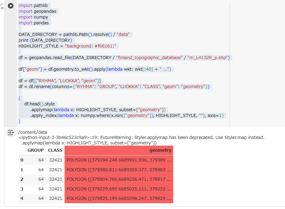
コードが長めですが、あまり気にしなくてよいかと。
肝心なのは、geometry列の中身が、POLYGON(....)となっていることです。
確かに、shapely.geometryオブジェクトになっています。
Input data: Finnish topographic database
In this lesson, we will work with the National Land Survey of Finland (NLS)/Maanmittauslaitos (MML) topographic database. - The data set is licensed under the NLS’ open data licence (CC BY 4.0). - The structure of the data is described in a separate Excel file. - Further information about file naming is available at fairdata.fi (this link relates to the 2018 issue of the topographic database, but is still valid).
For this lesson, we have acquired a subset of the topographic database as shapefiles from the Helsinki Region in Finland via the CSC’s Paituli download portal. You can find the files in data/finland_topographic_database/.
The Paituli spatial download service offers data from a long list of national institutes and agencies.
以降で使うデータの源泉についてです。興味があれば読み解いてもらえれば。
Read and explore geo-spatial data sets
Before we attempt to load any files, let’s not forget to defining a constant that points to our data directory:
ファイルを読み込むディレクトリのフルパスを定義しておきます。
import pathlib
NOTEBOOK_PATH = pathlib.Path().resolve()
DATA_DIRECTORY = NOTEBOOK_PATH / "data"
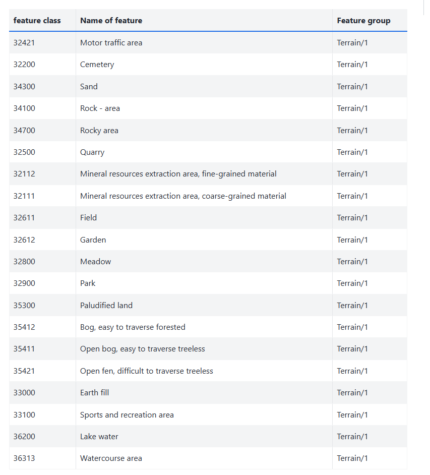
In this lesson, we will focus on terrain objects (Feature group: “Terrain/1” in the topographic database). The Terrain/1 feature group contains several feature classes.
Our aim in this lesson is to save all the Terrain/1 feature classes into separate files.
この後は、“Terrain/1”という地形オブジェクト(でしょうか、自信なし)のデータを使用します。
ひとまずは、いろいろな地物(例:池、公園)をfeature classという区分で格納している、と理解しておけばよいでしょう。
If you take a quick look at the data directory using a file browser, you will notice that the topographic database consists of many smaller files. Their names follow a strictly defined convention, according to this file naming convention, all files that we interested in (Terrain/1 and polygons) start with a letter m and end with a p.
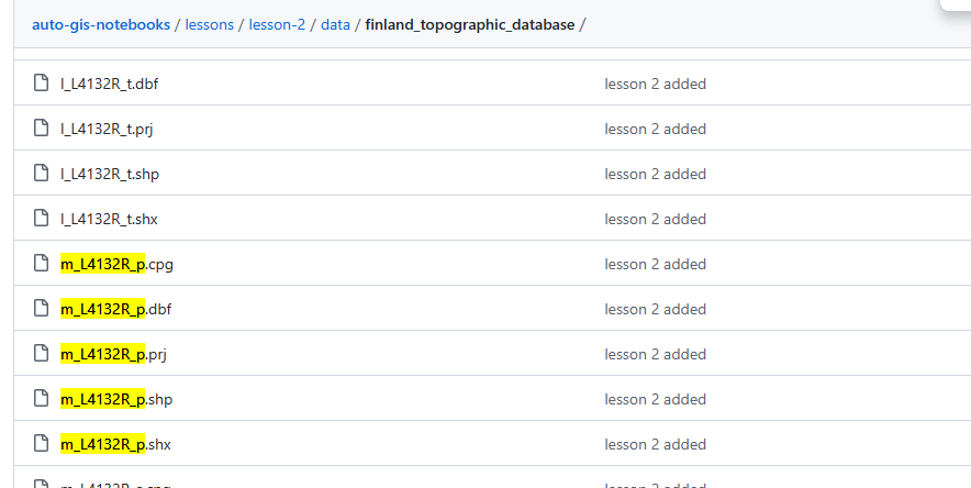
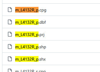
過程はすっ飛ばします。以下のファイルをアップロードします。
m_L4132R_p.cpg
m_L4132R_p.dbf
m_L4132R_p.prj
m_L4132R_p.shp
m_L4132R_p.shx
ファイルは、https://github.com/mopinfish/auto-gis-notebooks/tree/main/lessons/lesson-2/data/finland_topographic_database にあります。
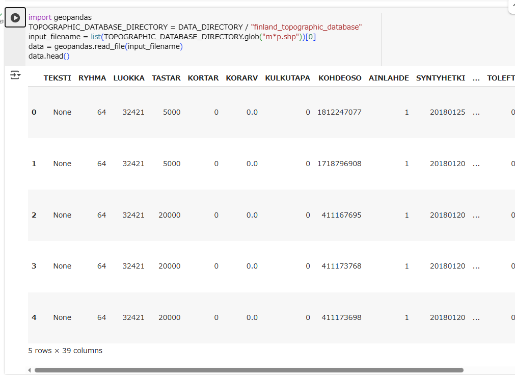
そして、上記のファイルを読み込みます。
import geopandas
TOPOGRAPHIC_DATABASE_DIRECTORY = DATA_DIRECTORY / "finland_topographic_database"
input_filename = list(TOPOGRAPHIC_DATABASE_DIRECTORY.glob("m*p.shp"))[0]
data = geopandas.read_file(input_filename)
data.head()
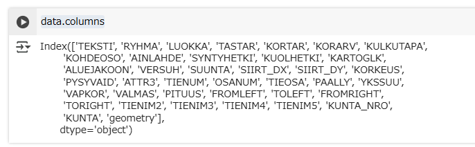
列を見てみましょう。
data.columns
列でフィルターします。
サンプルコード違い、フィルター後のGeoDataFrameの名前はdata_modifiedとしています。
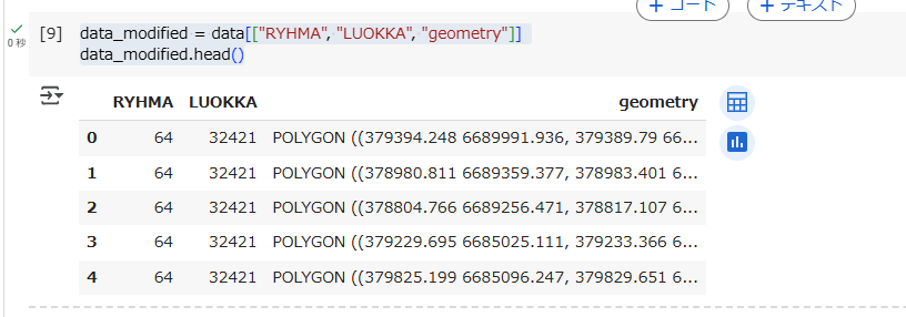
data_modified = data[["RYHMA", "LUOKKA", "geometry"]]
data_modified.head()
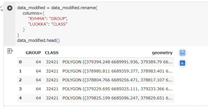
列名を変更します。
data_modified = data_modified.rename(
    columns={
        "RYHMA": "GROUP",
        "LUOKKA": "CLASS"
    }
)
data_modified.head()
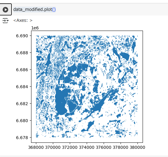
Explore the data set in a map:
As geographers, we love maps. But beyond that, it’s always a good idea to explore a new data set also in a map. To create a simple map of a geopandas.GeoDataFrame, simply use its plot() method. It works similar to pandas (see Lesson 7 of the Geo-Python course, but draws a map based on the geometries of the data set instead of a chart.
plot()メソッドでgeopandas.GeoDataFrameのデータを地図として表示できます。
data_modified.plot()
Geometries in geopandas
Geopandas takes advantage of shapely’s geometry objects. Geometries are stored in a column called geometry.
shapelyのgeometryオブジェクトは、geometryと呼ばれる列に格納されています。
data_modified.head()
Lo and behold, the geometry column contains familiar-looking values: Well-Known Text (WKT) strings. Don’t be fooled, they are, in fact, shapely.geometry objects (you might remember from last week’s lesson) that, when print()ed or type-cast into a str, are represented as a WKT string).
表示はWell-Known Text (WKT) ですが、実際はshapelyのgeometryオブジェクトです。
Since the geometries in a GeoDataFrame are stored as shapely objects, we can use shapely methods to handle geometries in geopandas.
Let’s take a closer look at (one of) the polygon geometries in the terrain data set, and try to use some of the shapely functionality we are already familiar with. For the sake of clarity, first, we’ll work with the geometry of the very first record, only:
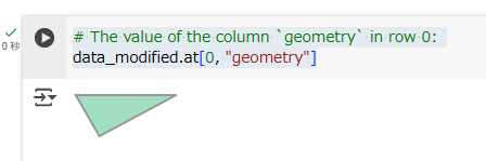
at()メソッドで1レコード目のgeometryを参照し、shapelyとしての機能を確認しましょう。
# The value of the column `geometry` in row 0:
data_modified.at[0, "geometry"]
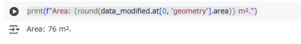
areaプロパティから面積を求めることができます。
print(f"Area: {round(data_modified.at[0, 'geometry'].area)} m².")
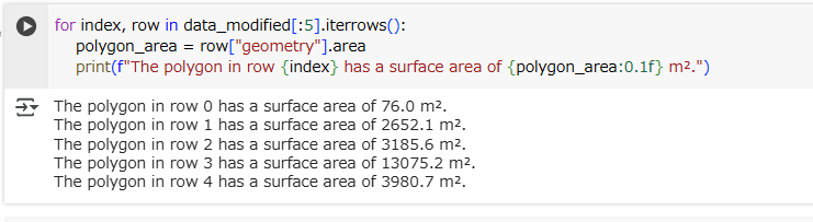
Let’s do the same for multiple rows, and explore different options of how to. First, use the reliable and tried iterrows() pattern we learned in lesson 6 of the Geo-Python course.
iterrows() メソッドで複数レコードまとめて処理しましょう。
for index, row in data_modified[:5].iterrows():
    polygon_area = row["geometry"].area
    print(f"The polygon in row {index} has a surface area of {polygon_area:0.1f} m².")
As you see, all pandas functions, such as the iterrows() method, are available in geopandas without the need to call pandas separately. Geopandas builds on top of pandas, and it inherits most of its functionality.
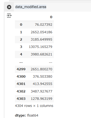
Of course the iterrows() pattern is not the most convenient and efficient way to calculate the area of many rows. Both GeoSeries (geometry columns) and GeoDataFrames have an area property:
pandasの機能はgeopandasでも同じように使えます。
ただ、複数レコードで、areaプロパティ処理するときに、iterrows() メソッドは最も有効な方法ではありません。
GeoSeriesやGeoDataFramesそのものがareaを持っています。
data_modified.area
上記は以下と同じ結果になります。
data_modified["geometry"].area
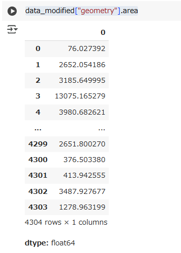
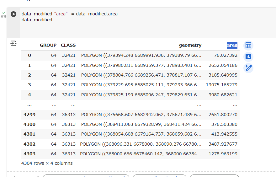
areaプロパティを別の列に外だしすることもできます。
長くなったのでここまでとします。続きます。