Automating GIS Processes 2024 写経 Lesson 4（Overlay analysis）

Overlay analyses are GIS operations in which two or more vector layers are combined to produce new geometries. Typical overlay operations include union, intersection, and difference - named after the result of the combination of two layers.

オーバーレイ分析＝2つ以上のベクターレイヤーを結合して新しいgeometryを作ること、です。典型的なオーバーレイ分析としては、結合、交差、差分があります。

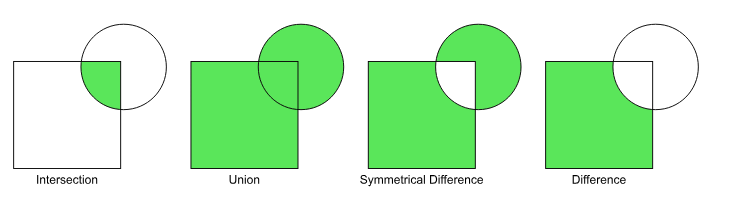
Figure: Spatial overlay with two input vector layers (rectangle, circle). The resulting vector layer is displayed in green. Source:QGIS documentation

矩形と円の２つのベクターレイヤーのオーバーレイについて、緑色で表示された箇所がその結果になります。詳細は、QGIS documentationを参照ください。

In this tutorial, we will carry out an overlay analysis to select those polygon cells of a grid dataset that lie within the city limits of Helsinki. For this exercise, we use two input data sets: a grid of statistical polygons with the travel time to the Helsinki railway station, covering the entire metropolitan area

(helsinki_region_travel_times_to_railway_station.gpkg) and a polygon data set (with one feature) of the area the municipality of Helsinki covers (helsinki_municipality.gpkg). Both files are in logically named subfolders of the DATA_DIRECTORY.

このチュートリアルでは、オーバーレイ分析を実行して、ヘルシンキの境界線内のグリッドデータセットのポリゴン群を選択します。２つのデータセットを使います。

１つはヘルシンキの駅への移動時間の統計情報のポリゴンです。これは中心市街地を網羅します。ファイル名は、helsinki_region_travel_times_to_railway_station.gpkgです。もう一つはヘルシンキの市町村を網羅する１つのポリゴンであるhelsinki_municipality.gpkgです。この２つのファイルはDATA_DIRECTORYのサブフォルダで、ファイル名と関連しているフォルダの中にあります。

import pathlib
NOTEBOOK_PATH = pathlib.Path().resolve()
DATA_DIRECTORY = NOTEBOOK_PATH / "data"

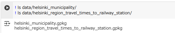
! ls data/helsinki_municipality/
! ls data/helsinki_region_travel_times_to_railway_station/

import geopandas

grid = geopandas.read_file(
    DATA_DIRECTORY
    / "helsinki_region_travel_times_to_railway_station"
    / "helsinki_region_travel_times_to_railway_station.gpkg"
)

helsinki = geopandas.read_file(
    DATA_DIRECTORY / "helsinki_municipality" / "helsinki_municipality.gpkg"
)

Let’s do a quick overlay visualization of the two layers:

では、可視化してみましょう。

# Plot the layers
ax = grid.plot(facecolor="gray")
helsinki.plot(ax=ax, facecolor="None", edgecolor="blue")

Here the grey area is the Travel Time Matrix - a data set that contains 13231 grid squares (13231 rows of data) that covers the Helsinki region, and the blue area represents the municipality of Helsinki. Our goal is to conduct an overlay analysis and select the geometries from the grid polygon layer that intersect with the Helsinki municipality polygon.

灰色のエリアは移動時間のマトリックスです。13231の場所（13231行のデータ）で、ヘルシンキの地域を網羅します。青色のエリアはヘルシンキの市町村です。
ゴールとしては、オーバーレイ分析を実施し、グリッドデータセットから、ヘルシンキの市町村のポリゴンと交差しているポリゴン群（geometry）群を選択することです。

When conducting overlay analysis, it is important to first check that the CRS of the layers match. The overlay visualization indicates that everything should be ok (the layers are plotted nicely on top of each other). However, let’s still check if the crs match using Python:

オーバーレイ分析をする際、最初にCRSがあっているかを確認することが重要です。オーバーレイの可視化で「すべてOK」（オーバーレイするレイヤー同士がうまくプロットされていること）を確認できます。が、CRSがあっているかも確認しましょう。

print(helsinki.crs)
print(grid.crs)

# Ensure that the CRS matches, if not raise an AssertionError
assert helsinki.crs == grid.crs, "CRS differs between layers!"

Indeed, they do. We are now ready to conduct an overlay analysis between these layers.

CRSはあっていますね。オーバーレイ分析を実施する準備ができました。

We will create a new layer based on grid polygons that intersect with our Helsinki layer. We can use a method overlay() of a GeoDataFrame to conduct the overlay analysis that takes as an input 1) second GeoDataFrame, and 2) parameter how that can be used to control how the overlay analysis is conducted (possible values are 'intersection', 'union', 'symmetric_difference', 'difference', and 'identity'):

前述の２つのレイヤーからポリゴン群からなるグリッドのレイヤーを作成します。GeoDataFrameのoverlay()メソッドを使います。引数の一つ目はもう一つのGeoDataFrame、２つ目のhowはどのオーバーレイ分析を使うかです。（'intersection'、'union'、'symmetric_difference'、'difference'、'identity'を設定します）

intersection = grid.overlay(helsinki, how="intersection")
intersection.plot(color="b")

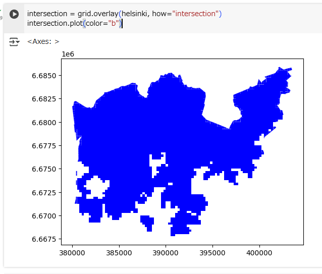
As a result, we now have only those grid cells that intersect with the Helsinki borders. If you look closely, you can also observe that the grid cells are clipped based on the boundary.

１つのグリッドができました。これはヘルシンキの境界線とintersect（交差）しています。

ax = grid.plot(facecolor="black", figsize=(20,20))  # グリッド、黒色
helsinki.plot(ax=ax, facecolor="None", edgecolor="red")  # ヘルシンキ市町村の境界線、赤色
intersection.plot(
    ax=ax, 
    color="gray", 
    alpha=0.7
) # intersectionの結果、白色

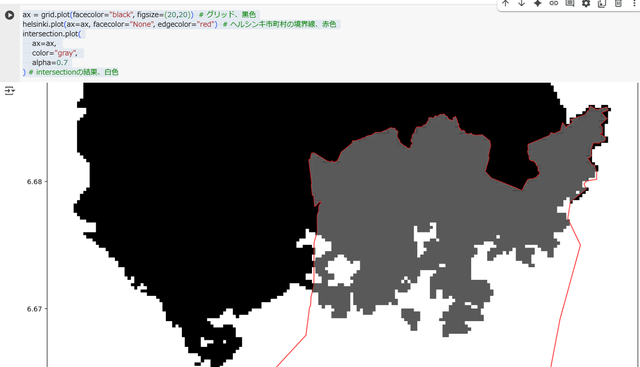
右端などを細かく見ると、intersectionは、グリッド（grid）から境界線（helsinki）によってクリップされたものであることがわかります。（グリッド：黒色、境界線：赤色、intersection：灰色）

• Whatabout the data attributes? Let’s see what we have:

データの属性値を見てみましょう。

intersection.head()

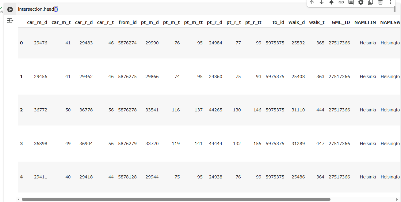
As we can see, due to the overlay analysis, the dataset contains the attributes from both input layers.

入力レイヤーにあった属性がこのグリッドに含まれていることがわかります。

Let’s save our result grid as a GeoPackage.

では、このグリッドをGeoPackageとしてファイル保存しましょう。

intersection.to_file(
    DATA_DIRECTORY / "intersection.gpkg",
    layer="travel_time_matrix_helsinki_region"
)

There are many more examples for different types of overlay analysis in Geopandas documentation where you can go and learn more.

オーバーレイ分析については、Geopandasのドキュメントにたくさんのサンプルがあり、学ぶことができます。

Reading and Writing GeoPackages with Multiple Layers
複数レイヤーでのGeoPackageの読み書きについて

GeoPackages are versatile spatial data formats that can store multiple layers in a single file. Here’s how you can work with them using Python and GeoPandas:

GeoPackageは多用途の空間データフォーマットで、複数のレイヤーを１つのファイルに格納できます。PythonとGeopandasで実現する方法は以下の通りです。

Writing Multiple Layers to a GeoPackage
Use the to_file method with the layer parameter to specify the name of each layer:

複数レイヤーを書き込むときは、to_file()メソッドを使います。その際、引数layerで書き込みたいレイヤーを指定します。

（ソースコードはgdf1とgdf2の定義を追加しています。）

from shapely.geometry import Point
import geopandas as gpd

d1 = {'col1': ['name1', 'name2'], 'geometry': [Point(1, 2), Point(2, 1)]}
gdf1= geopandas.GeoDataFrame(d1, crs="EPSG:4326")

d2 = {'col1': ['name1', 'name2'], 'geometry': [Point(11, 22), Point(22, 11)]}
gdf2= geopandas.GeoDataFrame(d2, crs="EPSG:4326")

# Example: Writing two layers
gdf1.to_file("example.gpkg", layer="layer1", driver="GPKG")
gdf2.to_file("example.gpkg", layer="layer2", driver="GPKG")

Reading Multiple Layers from a GeoPackage
List all available layers using fiona and then load specific ones:

複数レイヤーを読み込むときは、fionaでレイヤーのリストを作成し、そのリストを、read_file()メソッドの引数layerに指定します。

import geopandas as gpd
import fiona

# List layers in the GeoPackage
layers = fiona.listlayers("example.gpkg")
print(layers)  # Output: ['layer1', 'layer2']

# Read a specific layer
gdf1 = gpd.read_file("example.gpkg", layer="layer1")
print(gdf1)

gdf2 = gpd.read_file("example.gpkg", layer="layer2")
print(gdf2)

（補足） fionaパッケージがインストールされていない場合、以下のエラーがでます。こうなった場合は、! pip install fionaでインストールしましょう。

---------------------------------------------------------------------------
ModuleNotFoundError                       Traceback (most recent call last)
/tmp/ipython-input-26-1749735834.py in <cell line: 0>()
      1 import geopandas as gpd
----> 2 import fiona
      3 
      4 # List layers in the GeoPackage
      5 layers = fiona.listlayers("example.gpkg")

ModuleNotFoundError: No module named 'fiona'

Key Notes

• GeoPackages use the GPKG driver.
• They are ideal for combining multiple spatial datasets into a single file.
• It is a good habit to specify the layer name when working with multiple layers.

特記事項

• GeopandasはGPKGドライバーを使います
• 複数の空間データセットを、１つのファイルに格納することができます
• 複数レイヤーのデータを扱うときはレイヤーを特定することを習慣にすると良いでしょう

For more details, see the GeoPandas documentation.

詳細は、Geopandasのドキュメントを参照ください。