0. 目的
- MAR (missing at random) の仮定のもとでは、観測確率(の推定値)の逆数を重みとした一般化推定方程式(GEE)を用いることで、モデルが正しく推定されている場合に、パラメータの一致推定量を得ることができることが知られている1,2)
- そこで今回は、経時反復測定データを発生させ、
完全データおよびMARの下での欠測を発生させたデータをGEEを用いて解析し、パラメータの推定値が漸近的に真値に一致する様子をシミュレーションによって確認する
1.経時反復測定データの生成
データ生成モデル
- 0または1で表される、ある状態の観測値を経時的に観察した仮想データ
- i が被験者を表し、x が治療の有無を表す
- 治療の有無はランダムに 50 % の確率で各被験者に割り付ける
$logit[Pr(Y_{ij}=k|x_i,t)] = \beta_{0k} + \beta_{x}x_{i} + \beta_{t}I(t = j) + \beta_{xt}x_{i}I(t = j)$
$i$:被験者
$j$:時点($t_1, t_2, t_3, t_4$)
$y$:観察された状態(応答変数)
$k$:観察された状態のカテゴリ($0, 1$)
$x$:治療群($1$:治療群, $0$:プラセボ群)
$t$:時点
$I(t = j)$:時点 $j$ で観測されたデータであることを表す指示変数
観測確率モデル
- MARの仮定が真であるようなモデル:治療の有無と、当該観察時間以前の状態に依存して欠測が発生する
- 治療の有無と、当該観察時間の直前の観察状態を説明変数としたロジットモデルにより表現
$logit(p_t)=\gamma_{0}+\gamma_{1}Y_{t-1} + \gamma_2 x$
パラメータの真値
- パラメータの真値を次表のように設定し、データを発生させる
| $\beta_{01}$ | $\beta_{x}$ | $\beta_{t_1}$ | $\beta_{t_2}$ | $\beta_{t_3}$ | $\beta_{t_4}$ | $\beta_{xt_1}$ | $\beta_{xt_2}$ | $\beta_{xt_3}$ | $\beta_{xt_4}$ |
|---|---|---|---|---|---|---|---|---|---|
| $0.8$ | $0.5$ | $-0.4$ | $-0.2$ | $-0.1$ | $0$ | $-0.4$ | $-0.2$ | $-0.1$ | $0$ |
| $\gamma_0 $ | $\gamma_1$ | $\gamma_2$ |
|---|---|---|
| $2$ | $-0.1$ | $-0.2$ |
import numpy as np
import pandas as pd
from matplotlib import pyplot as plt
import statsmodels.api as sm
import statsmodels.formula.api as smf
from sklearn.linear_model import LogisticRegression
%matplotlib inline
from tqdm import tqdm

#class for generating data
class gen_data:

    def __gen_random_uniform(self, size, seed):
        np.random.seed(seed = seed)
        random = np.random.uniform(size = size)
        return random

    def __generate_prob_y1(self, time, treat):
        beta_0 = {"1" : 0.8}
        beta_x = 0.5
        beta_t = {"t1" : -0.4, "t2" : -0.2, "t3" : -0.1, "t4" : 0}
        beta_xt = {"t1" : -0.4, "t2" : -0.2, "t3" : -0.1, "t4" : 0}
        y = beta_0["1"] + beta_x * treat + beta_t[time] + treat * beta_xt[time]
        pr = np.exp(y) / (1 + np.exp(y))
        return pr

    def __generate_prob_obs(self, value, treat):
        gamma = {"0" : 2, "1" : - 0.1, "2" : -0.2}
        y = gamma["0"] + value * gamma["1"] + treat * gamma["2"]
        pr = np.exp(y) / (1 + np.exp(y))
        return pr

    def get_data(self, row = 1000, seed = 1):
        # set seed for random
        np.random.seed(seed = seed)

        # generate complete data
        data = {"id": np.arange(row),
                "treat": np.zeros(row),
                "t1": np.zeros(row),
                "t2": np.zeros(row),
                "t3": np.zeros(row),
                "t4": np.zeros(row),
                "random_treat" : self.__gen_random_uniform(size = row, seed = seed)
                }
        data["treat"][(data["random_treat"] <= 0.5)] = 1
        times = ["t1", "t2", "t3", "t4"]
        for time in times:
            treat = data["treat"]
            prob = self.__generate_prob_y1(time, treat)
            data[time] = np.random.binomial(1, prob)
        df_complete = pd.DataFrame(data)

        # generate missing data
        for time in times:
            treat = data["treat"]
            value = data[time]
            prob = self.__generate_prob_obs(value, treat)
            probs = np.random.binomial(1, prob)
            data[time][probs == 0] = -1
        df_missing = pd.DataFrame(data).replace(-1, np.nan)

        del df_complete["random_treat"]
        del df_missing["random_treat"]
        return df_complete, df_missing
重み付き GEE の実装
- 観測確率の推定値の逆数を重みとした weighted GEE を実装する
- 観測確率の推定モデルはロジスティック回帰
def analysis_GEE(formula, groups, cov_struct, data, weights=None, maxiter=10000):
    fam = sm.families.Binomial()
    mod = smf.gee(formula, groups="treat", data=data, cov_struct=cov_struct, family=fam, weights=weights)
    res = mod.fit(maxiter=maxiter)
    df_result = pd.DataFrame(res.conf_int()[0]).T
    return df_result

def calculate_weights_logisticRegression(X, y):
    for col in X.columns:
        X.loc[X[col].isnull()==True, col]='NA'
    X = pd.get_dummies(X)
    y[y == 1]='obs'
    y[y == 0]='obs'
    if len(y[y.isnull() == True]) == 0:
        # data has no missing values
        weights = np.ones(len(X.index))
    else:
        # data has missing values
        y[y.isnull() == True] = 'NA'
        X =  X.values
        y =  y.values[:,0]
        lr = LogisticRegression(solver='liblinear', max_iter=10000000)
        lr = lr.fit(X, y)
        y_pred = lr.predict_proba(X)
        probs = y_pred[:, 1]
        weights = 1 / probs
        weights[y == 'NA'] = 0
    return weights

# complete data analysis
def complete_analysis(df_complete, times):
    va = sm.cov_struct.Exchangeable()
    for i in range(len(times)):
        time = times[i]
        #implement GEE
        model = str(time) + " ~ treat"
        if len(times[0 : i ]) != 0:
            model = str(time) + " ~ treat +" + "+".join(times[0 : i ])
        df_tmp = analysis_GEE(formula=model, groups="treat", cov_struct=va, data=df_complete)
        df_tmp["time_point"] = time
        if i == 0:
            df = df_tmp
        else:
            df = pd.concat([df, df_tmp], sort=True)
    return df.reset_index(drop=True)

# missing data analysis
def missing_analysis(df_missing, times):
    va = sm.cov_struct.Exchangeable()
    for i in range(len(times)):
        time = times[i]
        # calculate weights for GEE by Logistic Regression
        X = pd.DataFrame(df_missing["treat"]).join(df_missing[times[0 : i]])
        y = pd.DataFrame(df_missing[time])
        weights = calculate_weights_logisticRegression(X, y)
        # implement weighted GEE
        model = str(time) + " ~ treat"
        if len(times[0 : i ]) != 0:
            model = str(time) + " ~ treat +" + "+".join(times[0 : i ])
        df_tmp = analysis_GEE(formula=model, groups="treat", cov_struct=va, data=df_missing, weights=weights)
        df_tmp["time_point"] = time
        if i == 0:
            df = df_tmp
        else:
            df = pd.concat([df, df_tmp], sort=True)
    return df.reset_index(drop=True)

def implement_analysis(row, times, seed = 1):
    # generate data
    df_complete, df_missing = gen_data().get_data(row = row, seed = seed)
    # complete data analysis
    df_result_complete = complete_analysis(df_complete, times)
    # missing data analysis
    df_result_missing = missing_analysis(df_missing, times)
    return df_result_complete, df_result_missing
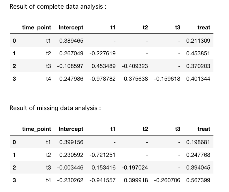
解析の実行例
- 300行のデータを生成
- GEE を用いた完全データの解析, weighted GEE を用いた欠測ありデータの解析を行う
times = ["t1", "t2", "t3", "t4"]
df_result_complete, df_result_missing = implement_analysis(row = 300, times = times, seed = 0)

print("\n")
for i in range(2):
    data = ["complete", "missing"][i]
    df = [df_result_complete, df_result_missing][i]
    print("Result of " + str(data) + " data analysis :")
    display(df.ix[:, ['time_point','Intercept','t1', 't2', 't3', 'treat']].replace(np.nan, "-"))
    print("\n")
解析結果
4. シミュレーションを実行する
- シミュレーション回数:100
- データ行数:100 - 5000(100刻みで増やしていく)
- データ行数 5000 に達した時点での推定パラメータを取得し、それらの平均を求める
simulation_time = 100
data_range = range(100, 5100, 100)

seeds = np.arange(len(data_range) * simulation_time)
seeds = np.reshape(seeds, (simulation_time, len(data_range)))

times = ["t1", "t2", "t3", "t4"]
trues = {"t1" : np.ones(len(data_range)) * 0.1,
         "t2" : np.ones(len(data_range)) * 0.3,
         "t3" : np.ones(len(data_range)) * 0.4,
         "t4" : np.ones(len(data_range)) * 0.5}

plt.figure(figsize=(15, 40))
plt.subplots_adjust(hspace=0.6)
param_comp = {"t1" : [], "t2" : [], "t3" : [], "t4" : []}
param_miss = {"t1" : [], "t2" : [], "t3" : [], "t4" : []}
for i in tqdm(range(simulation_time)):
    # implement simulation
    seed_range = seeds[i]
    treats_comp, treats_miss = simulate(data_range=data_range, seed_range=seed_range, times=times)
    for j in range(len(times)):
        time = times[j]
        param_comp[time].append(treats_comp[time][-1])
        param_miss[time].append(treats_miss[time][-1])
    # plot configurations
    subplot_area = (1, 4, 7, 10)
    for i in range(len(times)):
        time = times[i]
        area = subplot_area[i]
        plt.subplot(12, 1, area)
        plt.title("data : complete")
        plt.plot(data_range, treats_comp[time], color="limegreen", lw=0.5)
        plt.subplot(12, 1, area + 1)
        plt.title("data : missing")
        plt.plot(data_range, treats_miss[time], color="orangered", lw=0.5)
# plot configurations
for i in range(len(times)):
    time = times[i]
    area = subplot_area[i]
    plt.subplot(12, 1, area)
    plt.xlabel("number of data rows")
    plt.ylabel("coefficient of treat\ndata : complete")
    plt.plot(data_range, trues[time], label = "true", color="navy")
    plt.legend(borderaxespad=0.1)
    plt.subplot(12, 1, area + 1)
    plt.xlabel("number of data rows")
    plt.ylabel("coefficient of treat\ndata : missing")
    plt.plot(data_range, trues[time], label = "true", color="navy")
    plt.legend(borderaxespad=0.1)
plt.figtext(0.5,0.90, "Trace Plot of Simulated Parameters, Time Point : t1", ha="center", va="top", fontsize=24, color="black")
plt.figtext(0.5,0.71, "Trace Plot of Simulated Parameters, Time Point : t2", ha="center", va="top", fontsize=24, color="black")
plt.figtext(0.5,0.51, "Trace Plot of Simulated Parameters, Time Point : t3", ha="center", va="top", fontsize=24, color="black")
plt.figtext(0.5,0.315, "Trace Plot of Simulated Parameters, Time Point : t4", ha="center", va="top", fontsize=24, color="black")
print("\n")
plt.show()
# display result by dataframe
results = {}
for j in range(len(times)):
    time = times[j]
    results[j] = {"time point" : time, \
                          "true parameter" : trues[time][0], \
                          "mean of parameter(complete data)" : np.mean(param_comp[time]), \
                          "mean of parameter(missing data)" : np.mean(param_miss[time])}
print("Summary of result is below : ")
df = pd.DataFrame(results).T
df = df.ix[:, ['time point','true parameter','mean of parameter(complete data)', 'mean of parameter(missing data)']]
display(df)
シミュレーション結果
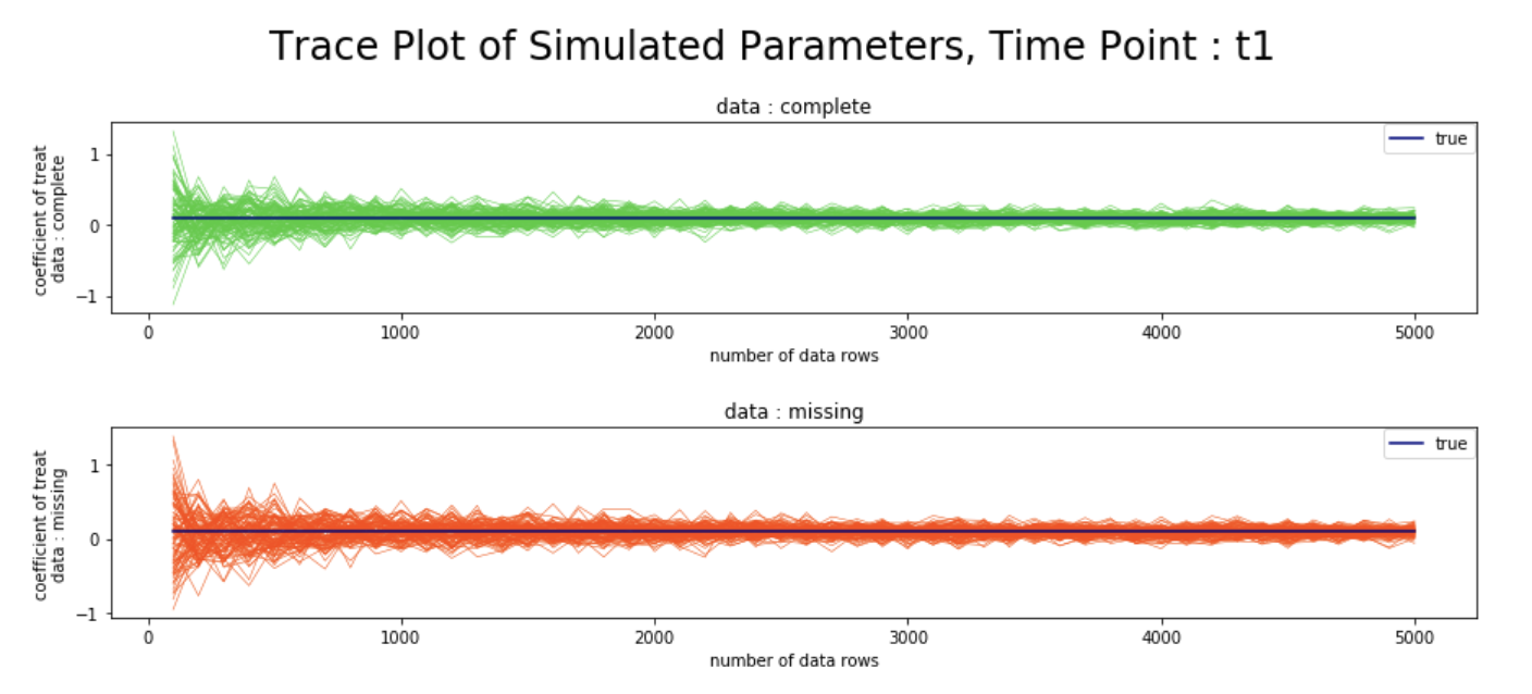
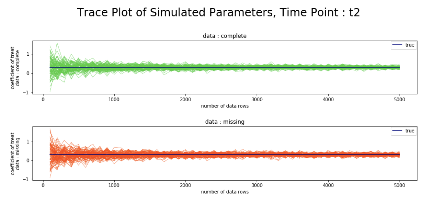
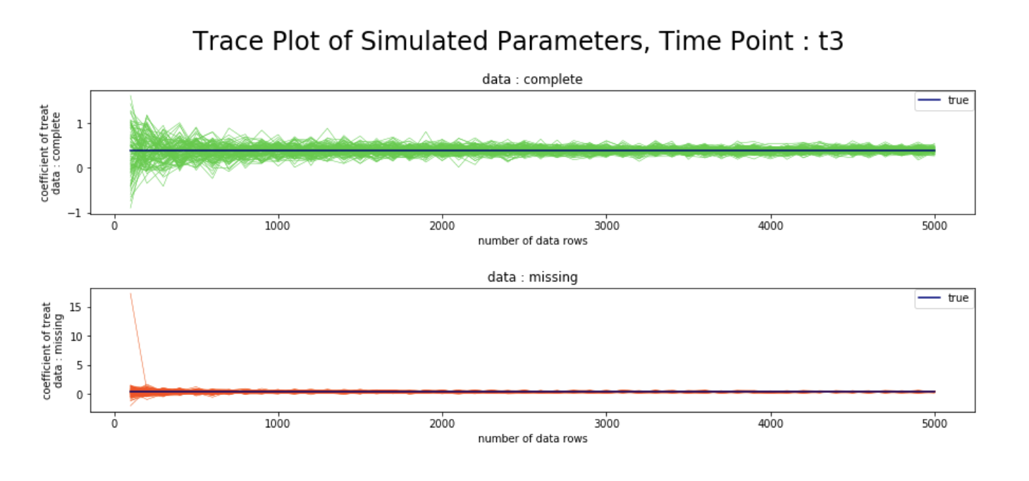
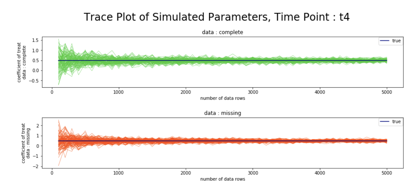
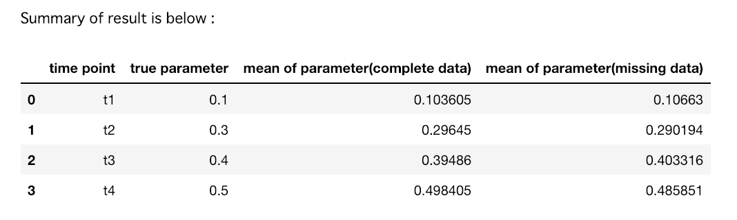
5. 結果
- 観測確率の推定値の逆数を重みとしたweighted GEEを用いることで、完全データと欠測データにおける、各時点での変数
treatの回帰係数が、データ数を増やすにつれて漸近的に真値へ収束する様子を、シミュレーションベースで確認することができた
6. Reference
- JM. Robins, A. Rotnitzky, LP. Zhao (1995) Analysis of Semiparametric Regression Models for Repeated Outcomes in the Presence of Missing Data, Journal of the American Statistical Association, 96, 106-121
- Preisser JS, Lohman KK, Rathouz PJ (2002) Performance of weighted estimating equations for longitudinal binary data with drop-outs missing at random, STATISTICS IN MEDICINE, 21, 3035-3054