機械学習 Rによる線形回帰

線形回帰：目的変数体説明変数のグラフを書くと先になる。

Rではlmコマンドを利用することで線形回帰分析を行うことができる。

lm(モデル関数、学習用データ)

目的: Tyrosineから絨毯の年齢を予測する。

1. データセットの読み込み

# データセットの読み込み
> carpet.data<-read.csv("http://www.stat.ufl.edu/~winner/data/carpet_age.csv", header=TRUE)

# 最後の2行は年齢が入ってないため削除
> carpet.data<-carpet.data[1:(nrow(carpet.data)-2),]

sample_id：絨毯ID
age:絨毯年齢
cys_acid: Cysteic Acidのレベル　※システイン酸
met:Methoionineのレベル　※メチニオン
tyr: Tyrosineのレベル　　　　　※チロシン

2.分類器（機械学習モデル）を作成

y  = a + bx

age  = a + b*tyr

# carpet.model.lm1にモデルオブジェクトが保存される
> carpet.model.lm1 <- lm(age ~ tyr, carpet.data)

3.予測値を取得

モデルオブジェクト(carpet.model.lm1)とデータ（carpet.data)をもとにして予測値を計算し、結果をapge.predicted.lm1列に格納。
predict関数で予測値を得る。

> carpet.data$age.predicted.lm1 <- predict(carpet.model.lm1,carpet.data)

# 予測値を確認
> head(carpet.data$age.predicted.lm1)
[1] 1772.335 1772.335 1682.160 1652.101 1652.101 1591.985

4.結果の可視化

• plot関数を使ってageとtyrの関係を可視化する。

> plot(x=carpet.data$tyr, y=carpet.data$age)

• 上のグラフに今回の線形器回帰分析で得られた予測値を赤点で可視化

> points(x=carpet.data$tyr, y=carpet.data$age.predicted.lm1,col="red")

• モデル直線を追加

> abline(a=carpet.model.lm1$coefficients[1],b=carpet.model.lm1$coefficients[2],col="blue")

# 以下でも同じ結果が得られる
> abline(carpet.model.lm1,col="blue")

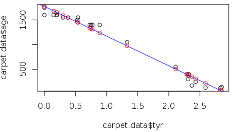
予測値はage = a + b x tyr上に載っている。

• 測定値 vs 予測値グラフ
  モデルによる予測がうまくいっていれば赤い直線（傾き1,切片0の直線）に近いところにプロットされる。

> plot(x=carpet.data$age,y=carpet.data$age.predicted.lm1)
> abline(a=0,b=1,col="red")

5.推定精度の検証

モデルでの予測精度を定量的に表す指標として決定係数がよく用いられる。
決定係数は目的変数の測定値と予測値を引数とする下記の関数で計算できる。
※決定係数はモデルの精度

決定係数は目的変数の測定値と予測値を引数とする下記の関数で計算できる。

> coef.det <- function(measured, predicted){
 1-sum((measured-predicted)^2) / sum((measured-mean(measured))^2)
 }

# モデルの決定係数を上記関数を使って求める
> coef.det(carpet.data$age,carpet.data$age.predicted.lm1)
[1] 0.9805863

決定係数が1に近いほどモデルの精度がいいことを意味する。

線形回帰モデルの場合は以下でも決定係数を取得可能

> summary(carpet.model.lm1)$r.squared
[1] 0.9805863

そんなに変わらない。

6.他のモデル関数を使ってみる

以下のモデル関数で試してみる。

y = a +bx + cx^2

# モデルオブジェクトを作成
> carpet.model.lm2 <- lm(age ~ poly(tyr,2), carpet.data)

# 予測値を求める
> carpet.data$age.predicted.lm2 <- predict(carpet.model.lm2,carpet.data)

# 決定係数を求める
> summary(carpet.model.lm2)$r.squared
[1] 0.98508