StanによるLatent parameter modelのポアソン分析ネタ。理論分布の名称はまちまちで、「ポアソン混合分布」ともいわれる。多峰性を示す報告データの統計解析をStanで推定したφ(..)メモメモ。(初実装2016-09)
ポアソン分布
この分布は単位時間あたりの事象がk回発生するときの確率分布。
歴史的には軍隊の落馬事故分析に始まり、報告、交通事故、味噌汁の具など幅広い事象の理論分布として用いられる。
$$
p_{poi}(X=x) = \frac{ \lambda^{x} e^{-\lambda}}{x!} (x = 1, 2,\cdots \infty: x \in \mathcal{N})
$$
uni modal であり、報告データの統計解析に多用される。
ある報告データで多峰性を示すモノが存在した。
古典的にはこの場合、複数のポアソン分布が混合している場合を考えるのが一般的と知った。混合率は測定困難な潜在因子と言われ、Latent parameter modelと言われる。
混合モデルと行った場合、$Poisson(\lambda)\times Binomial(\theta)$のようなモノを指す場合もあるようだ。 会社にあった70年代の本では "The finite mixture model" ともいうようだ。
一般に混合数は2と限らないが最小混合のbimodal distributionで、ポアソン分布の場合( mixture Poisson model)に限定して解いた。
正規混合分布の場合は、沢山の事例が紹介されているのでそちらを参考にできる。
Poisson Mixture Model の函数・尤度と問題
確率関数は下記になる。
\begin{align}
Pr(X=x|\pi, \lambda_1, \lambda_2) &= \mathbf{\pi} P_{pois}(X=x|\lambda_1) + \mathbf{(1-\pi)} P_{pois}(X=x|\lambda_2)
\end{align}
パラメータを$\boldsymbol{\theta} =\pi, \lambda_1, \lambda_2$ とした時、尤度関数は下記になる。
      L(\boldsymbol{\theta}) = f(y \mid \boldsymbol{\theta})  = \prod_{i=1}^{n} \Bigl\{
            \pi \Bigl(\frac{\lambda_{1}^{y_i}}{y_{i}!}e^{-\lambda_1} \Bigr)
    + (1 - \pi) \Bigl(\frac{\lambda_{2}^{y_i}}{y_{i}!}e^{-\lambda_2} \Bigr)\Bigr\}
ラベルスイッチ問題
この$\pi$が曲者で最初戸惑ったが、Stan Referenceの12.6. Inferences Supported by Mixtures項のInference under Label Switchingに事例がある。また、松浦のStanとRでベイズ統計モデリング (Wonderful R)には和文で解説がある。
- $\boldsymbol{\theta}=(0.3, 1, 4)$と$\boldsymbol{\theta}=(0.7, 1, 4)$が識別不能性
- (MCMCを複数チェインで行う場合、チェインごとに上記影響を受ける)
キチンと理解しておきたいが、力量たらず。Stanでは変数設定時に、simplex変数、大小関係を明示するコトがキー。 まぁ、1チェインで回せばスイッチの問題は避けられる。
Stanでのモデル定義
ポイントは、StanではLabel Switchingに対してparameter部での定義に於いてpositive_orderedとするvectorを宣言すれば良い。
data {
  int<lower=0> N;
  int          y[N];
}
parameters {
  real<lower=0,upper=1> R;
  positive_ordered[2]   lambda;  /*  MOST IMPORTANT SETTING */
}
transformed parameters{
}
model {
  R ~ beta(1, 1); // 無条件情報
  for (i in 1:N) {
    target += log_sum_exp(
                  log  (R) + poisson_lpmf(y[i] | lambda[1]),
                  log1m(R) + poisson_lpmf(y[i] | lambda[2]));
    }
}
generated quantities {
  vector[N] log_lik;
  for (i in 1:N) {
    // preferred Stan syntax as of version 2.10.0
    log_lik[i] = log_sum_exp(
                  log  (R) + poisson_lpmf(y[i] | lambda[1]),
                  log1m(R) + poisson_lpmf(y[i] | lambda[2]));
   }
}## PoiMixturePosOrd.stan
Refferenceによるとlog1m(R)も0演算を避けるためには重要だそうだ。
generated quantities部はWAICを使う時に必要な個別の尤度を出力させるためだ。混合数$k \ge 3$の時にモデル選択で用いられる予定に入れてあるが、本投稿では出番なしw
仮想データ作成関数
Rでポアソン混合モデル$(\pi=2)$のダミーデータ作成関数を作る。仮想データで推定。
makeMixtureDF <- function (r = 0.2, lambda1 = 0.2, lambda2 = 5, n = 100, plt = F, seed = 12341, def = T) {
    require("ggplot2");require("gridExtra")
    set.seed(seed)
    TXT <- base::sprintf("R = %0.1f,  Lambda1 = %0.1f, Lambda2 = %0.1f, N = %3.0f",
        r, lambda1, lambda2, n)
    y <- c(rpois(n * r, lambda1), rpois(n * (1 - r), lambda2))
    DFdat <- data.frame(x = 1:n, y = y, col = as.factor(c(rep("Lambda1",
        n * r), rep("Lambda2", n * (1 - r)))))
    if (plt == T) {
        p <- ggplot(DFdat, aes(x = x, y = y)) + geom_point(aes(colour = col))
        q <- ggplot(DFdat, aes(x = y, y = ..density.., colour = col)) +
            geom_density(adjust = 3, position = "identity") +
            labs(title = TXT) + geom_histogram(fill = "cornsilk",
            colour = "grey70", position = "identity", alpha = 0.5)
        grid.arrange(p, q, ncol = 1)
    }
    return(data = list(y = y, N = n, txt = TXT))
}
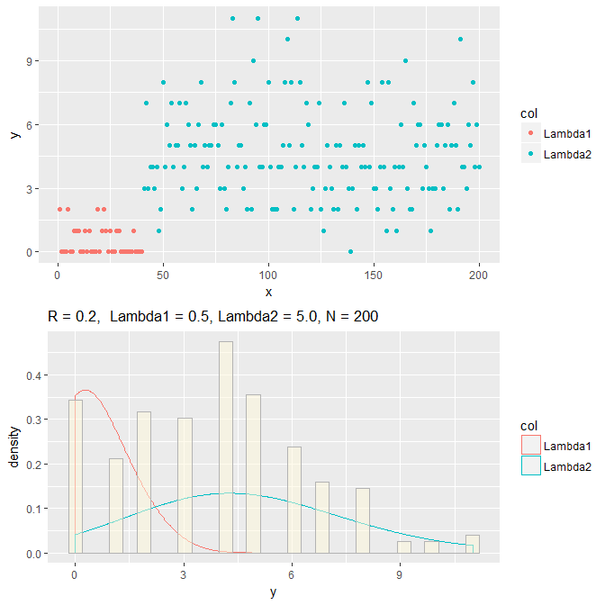
defaultと異なるパラメータを試したい時は、下記のようにする。ヒストグラムのbiningが甘いがご勘弁。
dat <- makeMixtureDF(r = 0.2, lambda1 = 0.5, lambda2 = 5.0, n = 200,plt=T)
標準的には次のように推定する。
modelPoiMixturePosOrd <- stan_model(model_code = PoiMixturePosOrd.stan)

fit1 <- sampling(modelPoiMixturePosOrdVer331,
                 data=list(y = dat$y, N = length(dat$y)),
                 iter = 10000,show_messages = F, control = list(adapt_delta = 0.9),
                 open_progress =F, chains =4 , verbose = F)
adapt_delta = 0.9は発散した時に適宜設定するらしい。結果は下記のように。
 Elapsed Time: 10.999 seconds (Warm-up)
               11.595 seconds (Sampling)
               22.594 seconds (Total)

> print(fit1c,pars=c("R", "lambda"))
Inference for Stan model: ceadd5ba78f82052921f72fc644a2af1.
4 chains, each with iter=10000; warmup=5000; thin=1;
post-warmup draws per chain=5000, total post-warmup draws=20000.

             mean se_mean   sd    2.5%     25%     50%     75%   97.5% n_eff Rhat
R            0.19    0.00 0.05    0.11    0.16    0.19    0.22    0.29  6071    1
lambda[1]    0.50    0.00 0.26    0.09    0.31    0.47    0.66    1.09  4360    1
lambda[2]    4.60    0.00 0.21    4.19    4.45    4.59    4.74    5.04 12269    1
サンプルデータ($\pi = 0.2, \lambda_1 = 0.5, \lambda_2 = 5.0$)を推定。
1万サンプルを4チェインで回した時、およそ23秒を要した(Core i5-1.9G)。
WAICはStan本家がパッケージを提供しているので利用が簡単。
> library('loo')
> log_lik <- extract_log_lik(fit1c)
> loo_1 <- loo(log_lik)
Computed from 20000 by 200 log-likelihood matrix

         Estimate   SE
elpd_loo   -469.7 10.3
p_loo         3.1  0.4
looic       939.3 20.6

All Pareto k estimates are good (k < 0.5)
See help('pareto-k-diagnostic') for details.
参考文献、その他
里村卓也著"マーケティング・モデル"にはマーケティングでの購買頻度モデルを解くために、この潜在クラスモデルをEMアルゴリズムで解く事例がある。
$\pi \ge 3$についてはEMで解く自身がないのでStanで実装する予定。
時系列分析の観点?
経済学の領域では、MARKOV SWITCHING MODELやマルコフ転移、状態空間モデルがキーワードのようだが、確率過程については勉強中。力量がたりない。
Rのlibrary("MswM")でも同様なことが出来るようだ。こちらのブログにRの事例がある。
先達の慧眼に恐れ入るところである。多謝。
蛇足
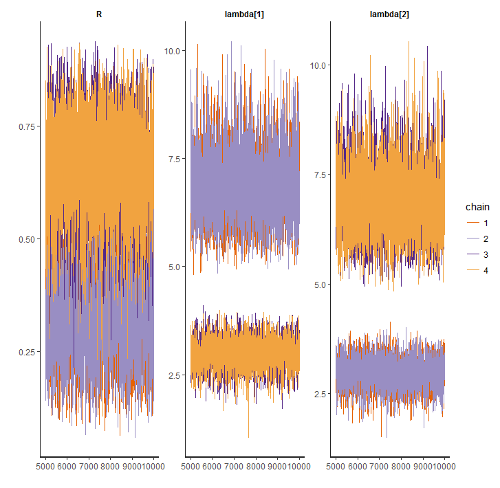
ラベル問題を解決しないと、rstan::traceplotで悲しい思いをする。
Inference for Stan model: 15c87bd3ba9a195d38618b1c8944c660.
4 chains, each with iter=10000; warmup=5000; thin=1;
post-warmup draws per chain=5000, total post-warmup draws=20000.

             mean se_mean   sd    2.5%     25%     50%     75%   97.5% n_eff Rhat
R            0.50    0.12 0.20    0.17    0.33    0.50    0.67    0.83     3 1.89
lambda[1]    4.92    1.38 2.02    2.42    2.99    4.45    6.79    8.20     2 3.66
lambda[2]    4.92    1.38 2.03    2.42    3.00    4.49    6.78    8.27     2 3.58
lp__      -468.87    0.02 1.27 -472.20 -469.45 -468.54 -467.93 -467.41  6949 1.00
推定結果は推定時の$\pi$を重みとした推定した$\lambda$の平均となり、さらにChainごとに異なるので複数Chainの平均となって結果がばらつく。最初悩んだ。
1chainでは推定できるが…エレガントではない。
> > Inference for Stan model: 15c87bd3ba9a195d38618b1c8944c660.
1 chains, each with iter=10000; warmup=5000; thin=1;
post-warmup draws per chain=5000, total post-warmup draws=5000.

             mean se_mean   sd    2.5%     25%     50%     75%   97.5% n_eff Rhat
R            0.34    0.00 0.11    0.15    0.26    0.33    0.41    0.58  1460    1
lambda[1]    6.85    0.02 0.80    5.54    6.28    6.77    7.34    8.61  1496    1
lambda[2]    2.98    0.01 0.33    2.30    2.76    2.99    3.20    3.60  1554    1
lp__      -468.85    0.03 1.26 -472.14 -469.46 -468.52 -467.93 -467.40  1888    1
以上