matplotlibでヒストグラムを書くにはhistを使う。
以下にいくつかの例を示す。
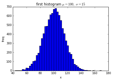
単純なヒストグラム
hist(データ、bins=ビン数)のように指定する。
title, labelはいつもの通りset_title, set_xlabel, set_ylabelを使う。
import numpy as np
import matplotlib.pyplot as plt

mu, sigma = 100, 15
x = mu + sigma * np.random.randn(10000)

fig = plt.figure()
ax = fig.add_subplot(1,1,1)

ax.hist(x, bins=50)
ax.set_title('first histogram $\mu=100,\ \sigma=15$')
ax.set_xlabel('x')
ax.set_ylabel('freq')
fig.show()
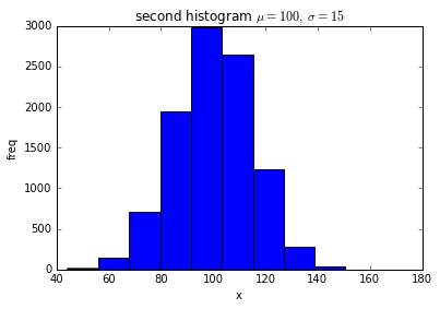
ビン数を10にした例(bins=10とする)。
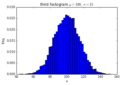
ヒストグラムを正規化する
normed=Trueとするとヒストグラムが正規化される。この時各ビンの頻度の合計は1.0となる。
import numpy as np
import matplotlib.pyplot as plt

mu, sigma = 100, 15
x = mu + sigma * np.random.randn(10000)

fig = plt.figure()
ax = fig.add_subplot(1,1,1)

ax.hist(x, bins=50, normed=True)
ax.set_title('third histogram $\mu=100,\ \sigma=15$')
ax.set_xlabel('x')
ax.set_ylabel('freq')
fig.show()
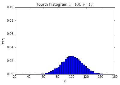
縦軸を固定する
ヒストグラムを比較する場合には縦軸が固定されていたほうが都合がよい場合がある。
この場合にはset_ylim(min, max)を使って縦軸を固定するとよい。
set_ylimを使わない場合は、データの頻度に応じてヒストグラム丁度いい具合に描画されるように縦軸が調整される。
import numpy as np
import matplotlib.pyplot as plt

mu, sigma = 100, 15
x = mu + sigma * np.random.randn(10000)

fig = plt.figure()
ax = fig.add_subplot(1,1,1)

ax.hist(x, bins=50, normed=True)
ax.set_title('fourth histogram $\mu=100,\ \sigma=15$')
ax.set_xlabel('x')
ax.set_ylabel('freq')
ax.set_ylim(0,0.1)
fig.show()
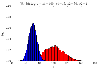
2つのヒストグラムを一枚のグラフに描画する
単純にhistを2回呼ぶ。
import numpy as np
import matplotlib.pyplot as plt

mu1, sigma1 = 100, 15
mu2, sigma2 = 70, 6
x1 = mu1 + sigma1 * np.random.randn(10000)
x2 = mu2 + sigma2 * np.random.randn(10000)

fig = plt.figure()
ax = fig.add_subplot(1,1,1)

ax.hist(x1, bins=50, normed=True, color='red')
ax.hist(x2, bins=50, normed=True, color='blue')
ax.set_title('fifth histogram $\mu1=100,\ \sigma1=15,\ \mu2=50,\ \sigma2=4$')
ax.set_xlabel('x')
ax.set_ylabel('freq')
ax.set_ylim(0,0.1)
fig.show()
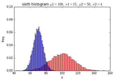
グラフを半透明にする
複数のヒストグラムを1枚のグラフに書いた場合に重なっている部分が隠れてしまう。
このときにグラフを半透明にすると少し見やすくなる。
半透明にする場合はパラメーターにalpha=0.5とする。
このとき値をalpha=1.0にするとグラフは不透明となりalphaを指定していないときと同じになり、
alpha=0.0とするとグラフは透明になりまったく見えなくなる。
import numpy as np
import matplotlib.pyplot as plt

mu1, sigma1 = 100, 15
mu2, sigma2 = 70, 6
x1 = mu1 + sigma1 * np.random.randn(10000)
x2 = mu2 + sigma2 * np.random.randn(10000)

fig = plt.figure()
ax = fig.add_subplot(1,1,1)

ax.hist(x1, bins=50, normed=True, color='red', alpha=0.5)
ax.hist(x2, bins=50, normed=True, color='blue',alpha=0.5)
ax.set_title('sixth histogram $\mu1=100,\ \sigma1=15,\ \mu2=50,\ \sigma2=4$')
ax.set_xlabel('x')
ax.set_ylabel('freq')
ax.set_ylim(0,0.1)
fig.show()
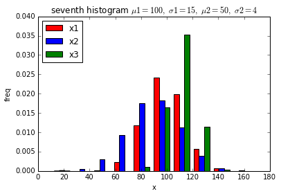
ヒストグラムを横に並べたいとき
複数のヒストグラムを1枚のグラフに描画するときに、比較しやすいようにビン単位でBarを横に並べたい場合がある。
この場合はデータを[x1, x2, x3]のようにlistにして、hist([x1, x2, x3])のようにする。
色やlabelも同様にlistにする。
import numpy as np
import matplotlib.pyplot as plt

mu1, sigma1 = 100, 15
mu2, sigma2 = 90, 20
mu3, sigma3 = 110, 10
x1 = mu1 + sigma1 * np.random.randn(10000)
x2 = mu2 + sigma2 * np.random.randn(10000)
x3 = mu3 + sigma3 * np.random.randn(10000)

fig = plt.figure()
ax = fig.add_subplot(1,1,1)

ax.hist([x1, x2, x3], bins=10, normed=True, color=['red', 'blue', 'green'], label=['x1', 'x2', 'x3'])
ax.set_title('seventh histogram $\mu1=100,\ \sigma1=15,\ \mu2=50,\ \sigma2=4$')
ax.set_xlabel('x')
ax.set_ylabel('freq')
ax.legend(loc='upper left')
fig.show()
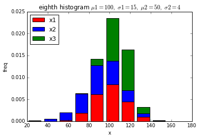
ヒストグラムを縦に積みあげたいとき
複数のヒストグラムを1枚のグラフに描画するときに、3つの合計で比較したい時にBarを縦に積みあげたい場合がある。
この場合はデータは横の時と同じようにhist([x1, x2, x3])のようにして、パラメーターにstacked=Trueと指定する。
import numpy as np
import matplotlib.pyplot as plt

mu1, sigma1 = 100, 15
mu2, sigma2 = 90, 20
mu3, sigma3 = 110, 10
x1 = mu1 + sigma1 * np.random.randn(10000)
x2 = mu2 + sigma2 * np.random.randn(10000)
x3 = mu3 + sigma3 * np.random.randn(10000)

fig = plt.figure()
ax = fig.add_subplot(1,1,1)

ax.hist([x1, x2, x3], bins=10, normed=True, color=['red', 'blue', 'green'], label=['x1', 'x2', 'x3'], histtype='bar', stacked=True)
ax.set_title('eighth histogram $\mu1=100,\ \sigma1=15,\ \mu2=50,\ \sigma2=4$')
ax.set_xlabel('x')
ax.set_ylabel('freq')
ax.legend(loc='upper left')
fig.show()
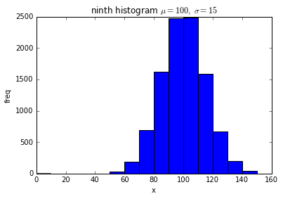
ビンの間隔を自分で指定したい場合
ビン数を指定するとデータの最大値、最小値に合わせて自動的にビンの間隔が決められる。
データの取りうる範囲でヒストグラムを作成したいときなど、データに依存せずビンの間隔を自分で決めたい時がある。
その場合はビンのedgeのlistを作成し、パラメーターでbins=edgesのように指定する。
ビンのedgeとは、ビンの下限値、または上限値のことを指し、例えばビンの数が10個の場合はedgeの数は11個となる。
import numpy as np
import matplotlib.pyplot as plt

mu, sigma = 100, 15
x = mu + sigma * np.random.randn(10000)

fig = plt.figure()
ax = fig.add_subplot(1,1,1)
edges = range(0,160,10)
n, bins, patches = ax.hist(x, bins=edges)
ax.set_title('ninth histogram $\mu=100,\ \sigma=15$')
ax.set_xlabel('x')
ax.set_ylabel('freq')
fig.show()
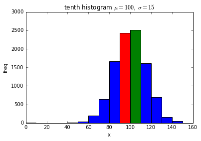
ヒストグラムのデータを取得したい時
グラフの描画とその時のヒストグラムの頻度データの取得を同時に行いたい場合、
n, bins, pathces = ax.hist(x, ...)のようにhistの戻り値で頻度データを取得する。
戻り値のpatchesとは?
patchesはlistでその中身は、描画したヒストグラムのビン毎のobjectである。
ヒストグラムのビンのobjectのpropertyを変えてあげると、その部分だけ色を変更することができる。
import numpy as np
import matplotlib.pyplot as plt

mu, sigma = 100, 15
x = mu + sigma * np.random.randn(10000)

fig = plt.figure()
ax = fig.add_subplot(1,1,1)
edges = range(0,160,10)
n, bins, patches = ax.hist(x, bins=edges)
ax.set_title('tenth histogram $\mu=100,\ \sigma=15$')
ax.set_xlabel('x')
ax.set_ylabel('freq')
patches[9].set_facecolor('red')
patches[10].set_facecolor('green')
fig.show()