ラビットチャレンジ 機械学習

０章　機械学習のイメージ

機械学習は、問題設定もしくは学習シナリオ（教師あり学習、教師なし学習、半教師あり学習、強化学習）をコンピュータに与え、それが解けるようするために訓練させるイメージです。

教師あり学習

入力データと出力データから、そのデータを説明できる評価関数を作成する手法
分類と回帰がある。

分類：SVM（サポートベクターマシーン）、ランダムフォレスト
回帰：線形回帰、ランダムフォレスト

長所	短所
特徴量を自動作成	入力データにノウハウが必要
ビックデータに生かせる	大量のデータが必要
一部に限定することで人間の能力を凌駕	学習した以上の結果は得られない
	結果の理由がブラックボックス

教師なし学習

入力データのみから、そのデータを説明できる評価関数を作成する手法
クラスタリングと次元削減がある

クラスタリング：$k$平均法、階層クラスタリング、自己組織化写像
次元削減：主成分分析（PCA）、因子分析

強化学習

ある環境下で、目的とする報酬を最大化するために、どのような行動をとるべきかを確立する手法

0.1 機械学習の定義

トム・ミッチェルによる機械学習の定義（1997）は次の通り

コンピュータプログラムは、タスクTを性能評価Pで測定し、その性能が経験Eにより改善される場合、タスクTおよび性能指標Pに関して経験Eから学習すると言われている

タスクT：アプリケーションにさせたいこと
性能評価P：予想と実際の差
経験E：データ

0.2 機械学習の前に

機械学習や深層学習を積極的に利用したい気持ちは分かるが、問題の解決に必ずしも機械学習や深層学習を使う必要はない。機械学習や深層学習にもデメリットがあり、使わない方が効率が良い場合も往々にしてある。

0.2.1 機械学習・深層学習のデメリット

機械学習や深層学習には、応用数学（線形代数、微分積分、確率統計及び情報理論）の知識が必要である。
そのため開発ができたとしても、機械学習・深層学習の知識がない人がトラブルを起こした場合、解決することができない。

0.2.2 機械学習・深層学習に必要なデータの前処理

集めたデータ（ローデータ）はそのまま使えるとことは少なく、欠損値や異常値に対する適切なクレンジング処理が必要である。

第１章　線形回帰モデル

まずは、機械学習モデルの中で代表的な線形回帰モデルを考察する。
線形回帰は教師あり学習の１つであり、目的変数が説明変数の係数に対して線形なモデルを学習するものである。
線形回帰では訓練データに適合する回帰係数を学習する際、２乗誤差の最小化を行う

1.1 回帰問題

教師あり学習の１つであり、ざっくり言うと関数近似問題。
ある入力値（離散値または連続値）から、連続値の出力を予測する問題。

• 直線（１次関数）で予想する場合：線形回帰（Linear regression）
• 曲線（１次関数以外）で予想する場合：非線形回帰（Nonlinear regression）

回帰は予測のみならず、ランキング問題も解くことができるが、おススメしない。
回帰問題を解くことと、ランキング問題を解くことを比較すると回帰問題を解く方が難しい。
難しい問題（回帰問題）を解くことで、簡単な問題（ランキング問題）を解くべきではない。
参考：Vapnik（バプニック）の原理
VapnikはSVM（サポートベクターマシーン）を提唱した人

1.2 回帰問題で扱うデータ

• 入力データ

　各要素の説明変数または特徴量と呼ぶ
　$m$次元のベクトル（$m=1$の場合は、スカラー）

$$x=(x_1,x_2,x_3,\cdots,x_m)^T\in\mathbb{R^m}$$

　$m=1$の場合
$$x\in\mathbb{R}$$

$\mathbb{R}$；実数全体
慣例としてベクトルは太字で書く。$T$は転値

• 出力データ （出力を複数にすることはできる。マルチタスク学習が近い。） 　目的変数と呼ぶ（スカラー値である）

$$y\in\mathbb{R}$$

説明変数（$x\in\mathbb{R^m}$）を使って、目的変数（$y\in\mathbb{R}$）を予測できるようする。
教師データ　{ $(x_i,y_i);i=1,2,3,\cdots,n $ }
回帰問題の具体例には、住宅価格の予測や来場者の予測などがある。

ボストンの住宅価格データ（Boston Housingデータセット：The Boston house-price data）の予測を例に挙げた場合
説明変数（$x\in\mathbb{R^m}$）：１３変数（犯罪率、敷地面積、産業、川の隣、環境、部屋数、築年数、距離、道路、税金、生徒と先生、黒人、低所得）
目的変数（$y\in\mathbb{R}）$：住宅価格

注：ボストンの住宅価格データ（Boston Housingデータセット
1970年代後半における（米国マサチューセッツ州にある）ボストンの住宅価格の表形式データセット（＝構造化データセット）のこと。（家賃の予想をする。）

1.3 線形回帰モデルのパラメータ

線形回帰のモデルの推定するべき未知のパラメータ$w$は
$$w=(w_1,w_2,w_3,\cdots,w_m)^T\in\mathbb{R^m}$$

切片を$w_0$とする。（切片をバイアス項ともいう）

なお、回帰問題のゴールは、{ $(x_i,y_i);i=1,2,3,\cdots,n $ } を用いて、
うまいパラメータ $w=(w_1,w_2,w_3,\cdots,w_n)$ を求めること。
最終的には、教師データにはない $x$ を持ってきて、その入力を線形回帰モデルに入力することで、出力を得る。

1.4 線形結合

予測値を $\hat{y}\in\mathbb{R}$ とすると、（慣例として予測値にはハット^を付ける）
（目的変数 $y\in\mathbb{R}$ と混同しないため、予測値を $\hat{y}\in\mathbb{R}$ とする）

\begin{eqnarray}
\hat{y}&=&w^Tx+w_0=(w_1,w_2,w_3,\cdots,w_m)
\begin{pmatrix}
x_1\\
x_2\\
x_3\\
\vdots \\
x_m
\end{pmatrix}+w_0\\
&=& w_1x_1+w_2x_2+w_3x_3+\cdots+w_mx_m+w_0\\
&=& \sum_{k=1}^m x_k w_k+w_0
\end{eqnarray}

と表すことができる。

1.5 単回帰モデル

単回帰 ⇒　直線　⇒　1次元のイメージ
説明変数が1次元 （$w=w_1$）の場合を単回帰といい、直線の式で表される
データについては、回帰直線に誤差 $\epsilon$ を考慮すると

$$y=w_0+w_1x_1+\epsilon$$
$y$：目的変数、 $w_0$：切片、 $w_1$：回帰係数、 $x_1$：説明変数、 $\epsilon$：誤差

$x_1$と$y$が既知のため、$\epsilon$ が最小になるように、パラメータ $w_0$と$w_1$ を設定すればよい。

1.6 重回帰モデル

単回帰 ⇒　局面・超平面　⇒　$m$次元のイメージ
説明変数が多次元（$m$次元（$1\leqq m\in\mathbb{N}$））の場合を重回帰という。
データについては、回帰直線に誤差 $\epsilon$ を考慮すると
$$y=w_0+w_1x_1+w_2x_2+w_3x_3+\cdots+w_mx_m+\epsilon=w_0+\sum_{k=1}^m w_kx_k+\epsilon$$

$y$：目的変数、 $w_0$：切片、 $\epsilon$：誤差、
$w_1,w_2,w_3\cdots ,w_m$：回帰係数、
$x_1,x_2,x_3\cdots ,x_m$：説明変数

1.7 パラメータの推定

1.7.1 平均二乗誤差（残差平方和）（Mean Squared Error）

データとモデル出力の誤差を二乗した後、平均を取ったもの
小さいほど直線とデータの距離が近い
頭文字をとってMSEで表す。
データは既知のもので、パラメータは未知である。

$$MSE_{\rm train}=\frac{1}{n_{\rm train}}\sum_{k=1}^{n_{\rm train}}\Big(\hat{y_k}-y_k\Big)^2$$

1.7.2 最小二乗法

学習データの平均二乗誤差を最小とするパラメータを探索する方法
学習データの平均二乗誤差の最小化は、その勾配が0になる点を求めれば良い

MSEを最小にするような $w\in\mathbb{R^m}$
$$\hat{w}=\arg \min_{w\in\mathbb{R^{m+1}}}MSE_{\rm train}$$

$w$に対して微分したものが0となる$w$の点を求める。つまり勾配が0になる点を求める。
$$\frac{\partial}{\partial w}MSE_{\rm train}=0$$

第１章　線形回帰のハンズオン

ボストンの住宅データセットを線形回帰モデルで分析（適切な査定結果が必要）

課題：部屋数が4で犯罪率が0.3の物件はいくらになるか？

必要なモジュールとデータのインポート

# from モジュール名 import クラス名（もしくは関数名や変数名）
from sklearn.datasets import load_boston
from pandas import DataFrame
import numpy as np

# ボストンデータを"boston"というインスタンスにインポート
boston = load_boston()

# インポートしたボストンデータを確認(data / target / feature_names / DESCR)
print(boston)

{'data': array([[6.3200e-03, 1.8000e+01, 2.3100e+00, ..., 1.5300e+01, 3.9690e+02,
4.9800e+00],
[2.7310e-02, 0.0000e+00, 7.0700e+00, ..., 1.7800e+01, 3.9690e+02,
9.1400e+00],
[2.7290e-02, 0.0000e+00, 7.0700e+00, ..., 1.7800e+01, 3.9283e+02,
4.0300e+00],
...,
[6.0760e-02, 0.0000e+00, 1.1930e+01, ..., 2.1000e+01, 3.9690e+02,
5.6400e+00],
[1.0959e-01, 0.0000e+00, 1.1930e+01, ..., 2.1000e+01, 3.9345e+02,
6.4800e+00],
[4.7410e-02, 0.0000e+00, 1.1930e+01, ..., 2.1000e+01, 3.9690e+02,
7.8800e+00]]), 'target': array([24. , 21.6, 34.7, 33.4, 36.2, 28.7, 22.9, 27.1, 16.5, 18.9, 15. ,
18.9, 21.7, 20.4, 18.2, 19.9, 23.1, 17.5, 20.2, 18.2, 13.6, 19.6,
15.2, 14.5, 15.6, 13.9, 16.6, 14.8, 18.4, 21. , 12.7, 14.5, 13.2,
13.1, 13.5, 18.9, 20. , 21. , 24.7, 30.8, 34.9, 26.6, 25.3, 24.7,
21.2, 19.3, 20. , 16.6, 14.4, 19.4, 19.7, 20.5, 25. , 23.4, 18.9,
35.4, 24.7, 31.6, 23.3, 19.6, 18.7, 16. , 22.2, 25. , 33. , 23.5,
19.4, 22. , 17.4, 20.9, 24.2, 21.7, 22.8, 23.4, 24.1, 21.4, 20. ,
20.8, 21.2, 20.3, 28. , 23.9, 24.8, 22.9, 23.9, 26.6, 22.5, 22.2,
23.6, 28.7, 22.6, 22. , 22.9, 25. , 20.6, 28.4, 21.4, 38.7, 43.8,
33.2, 27.5, 26.5, 18.6, 19.3, 20.1, 19.5, 19.5, 20.4, 19.8, 19.4,
21.7, 22.8, 18.8, 18.7, 18.5, 18.3, 21.2, 19.2, 20.4, 19.3, 22. ,
20.3, 20.5, 17.3, 18.8, 21.4, 15.7, 16.2, 18. , 14.3, 19.2, 19.6,
23. , 18.4, 15.6, 18.1, 17.4, 17.1, 13.3, 17.8, 14. , 14.4, 13.4,
15.6, 11.8, 13.8, 15.6, 14.6, 17.8, 15.4, 21.5, 19.6, 15.3, 19.4,
17. , 15.6, 13.1, 41.3, 24.3, 23.3, 27. , 50. , 50. , 50. , 22.7,
25. , 50. , 23.8, 23.8, 22.3, 17.4, 19.1, 23.1, 23.6, 22.6, 29.4,
23.2, 24.6, 29.9, 37.2, 39.8, 36.2, 37.9, 32.5, 26.4, 29.6, 50. ,
32. , 29.8, 34.9, 37. , 30.5, 36.4, 31.1, 29.1, 50. , 33.3, 30.3,
34.6, 34.9, 32.9, 24.1, 42.3, 48.5, 50. , 22.6, 24.4, 22.5, 24.4,
20. , 21.7, 19.3, 22.4, 28.1, 23.7, 25. , 23.3, 28.7, 21.5, 23. ,
26.7, 21.7, 27.5, 30.1, 44.8, 50. , 37.6, 31.6, 46.7, 31.5, 24.3,
31.7, 41.7, 48.3, 29. , 24. , 25.1, 31.5, 23.7, 23.3, 22. , 20.1,
22.2, 23.7, 17.6, 18.5, 24.3, 20.5, 24.5, 26.2, 24.4, 24.8, 29.6,
42.8, 21.9, 20.9, 44. , 50. , 36. , 30.1, 33.8, 43.1, 48.8, 31. ,
36.5, 22.8, 30.7, 50. , 43.5, 20.7, 21.1, 25.2, 24.4, 35.2, 32.4,
32. , 33.2, 33.1, 29.1, 35.1, 45.4, 35.4, 46. , 50. , 32.2, 22. ,
20.1, 23.2, 22.3, 24.8, 28.5, 37.3, 27.9, 23.9, 21.7, 28.6, 27.1,
20.3, 22.5, 29. , 24.8, 22. , 26.4, 33.1, 36.1, 28.4, 33.4, 28.2,
22.8, 20.3, 16.1, 22.1, 19.4, 21.6, 23.8, 16.2, 17.8, 19.8, 23.1,
21. , 23.8, 23.1, 20.4, 18.5, 25. , 24.6, 23. , 22.2, 19.3, 22.6,
19.8, 17.1, 19.4, 22.2, 20.7, 21.1, 19.5, 18.5, 20.6, 19. , 18.7,
32.7, 16.5, 23.9, 31.2, 17.5, 17.2, 23.1, 24.5, 26.6, 22.9, 24.1,
18.6, 30.1, 18.2, 20.6, 17.8, 21.7, 22.7, 22.6, 25. , 19.9, 20.8,
16.8, 21.9, 27.5, 21.9, 23.1, 50. , 50. , 50. , 50. , 50. , 13.8,
13.8, 15. , 13.9, 13.3, 13.1, 10.2, 10.4, 10.9, 11.3, 12.3, 8.8,
7.2, 10.5, 7.4, 10.2, 11.5, 15.1, 23.2, 9.7, 13.8, 12.7, 13.1,
12.5, 8.5, 5. , 6.3, 5.6, 7.2, 12.1, 8.3, 8.5, 5. , 11.9,
27.9, 17.2, 27.5, 15. , 17.2, 17.9, 16.3, 7. , 7.2, 7.5, 10.4,
8.8, 8.4, 16.7, 14.2, 20.8, 13.4, 11.7, 8.3, 10.2, 10.9, 11. ,
9.5, 14.5, 14.1, 16.1, 14.3, 11.7, 13.4, 9.6, 8.7, 8.4, 12.8,
10.5, 17.1, 18.4, 15.4, 10.8, 11.8, 14.9, 12.6, 14.1, 13. , 13.4,
15.2, 16.1, 17.8, 14.9, 14.1, 12.7, 13.5, 14.9, 20. , 16.4, 17.7,
19.5, 20.2, 21.4, 19.9, 19. , 19.1, 19.1, 20.1, 19.9, 19.6, 23.2,
29.8, 13.8, 13.3, 16.7, 12. , 14.6, 21.4, 23. , 23.7, 25. , 21.8,
20.6, 21.2, 19.1, 20.6, 15.2, 7. , 8.1, 13.6, 20.1, 21.8, 24.5,
23.1, 19.7, 18.3, 21.2, 17.5, 16.8, 22.4, 20.6, 23.9, 22. , 11.9]), 'feature_names': array(['CRIM', 'ZN', 'INDUS', 'CHAS', 'NOX', 'RM', 'AGE', 'DIS', 'RAD',
'TAX', 'PTRATIO', 'B', 'LSTAT'], dtype='<U7'), 'DESCR': ".. _boston_dataset:\n\nBoston house prices dataset\n---------------------------\n\n*Data Set Characteristics:* \n\n :Number of Instances: 506 \n\n :Number of Attributes: 13 numeric/categorical predictive. Median Value (attribute 14) is usually the target.\n\n :Attribute Information (in order):\n - CRIM per capita crime rate by town\n - ZN proportion of residential land zoned for lots over 25,000 sq.ft.\n - INDUS proportion of non-retail business acres per town\n - CHAS Charles River dummy variable (= 1 if tract bounds river; 0 otherwise)\n - NOX nitric oxides concentration (parts per 10 million)\n - RM average number of rooms per dwelling\n - AGE proportion of owner-occupied units built prior to 1940\n - DIS weighted distances to five Boston employment centres\n - RAD index of accessibility to radial highways\n - TAX full-value property-tax rate per $10,000\n - PTRATIO pupil-teacher ratio by town\n - B 1000(Bk - 0.63)^2 where Bk is the proportion of blacks by town\n - LSTAT % lower status of the population\n - MEDV Median value of owner-occupied homes in $1000's\n\n :Missing Attribute Values: None\n\n :Creator: Harrison, D. and Rubinfeld, D.L.\n\nThis is a copy of UCI ML housing dataset.\nhttps://archive.ics.uci.edu/ml/machine-learning-databases/housing/\n\n\nThis dataset was taken from the StatLib library which is maintained at Carnegie Mellon University.\n\nThe Boston house-price data of Harrison, D. and Rubinfeld, D.L. 'Hedonic\nprices and the demand for clean air', J. Environ. Economics & Management,\nvol.5, 81-102, 1978. Used in Belsley, Kuh & Welsch, 'Regression diagnostics\n...', Wiley, 1980. N.B. Various transformations are used in the table on\npages 244-261 of the latter.\n\nThe Boston house-price data has been used in many machine learning papers that address regression\nproblems. \n \n.. topic:: References\n\n - Belsley, Kuh & Welsch, 'Regression diagnostics: Identifying Influential Data and Sources of Collinearity', Wiley, 1980. 244-261.\n - Quinlan,R. (1993). Combining Instance-Based and Model-Based Learning. In Proceedings on the Tenth International Conference of Machine Learning, 236-243, University of Massachusetts, Amherst. Morgan Kaufmann.\n", 'filename': 'D:\Anaconda3\lib\site-packages\sklearn\datasets\data\boston_house_prices.csv'}

# DESCR変数の中身を確認
print(boston['DESCR'])

出力結果は次の通り

.. _boston_dataset:

Boston house prices dataset

Data Set Characteristics:

:Number of Instances: 506

:Number of Attributes: 13 numeric/categorical predictive. Median Value (attribute 14) is usually the target.

:Attribute Information (in order):
- CRIM per capita crime rate by town
- ZN proportion of residential land zoned for lots over 25,000 sq.ft.
- INDUS proportion of non-retail business acres per town
- CHAS Charles River dummy variable (= 1 if tract bounds river; 0 otherwise)
- NOX nitric oxides concentration (parts per 10 million)
- RM average number of rooms per dwelling
- AGE proportion of owner-occupied units built prior to 1940
- DIS weighted distances to five Boston employment centres
- RAD index of accessibility to radial highways
- TAX full-value property-tax rate per $10,000
- PTRATIO pupil-teacher ratio by town
- B 1000(Bk - 0.63)^2 where Bk is the proportion of blacks by town
- LSTAT % lower status of the population
- MEDV Median value of owner-occupied homes in $1000's

:Missing Attribute Values: None

:Creator: Harrison, D. and Rubinfeld, D.L.

This is a copy of UCI ML housing dataset.
https://archive.ics.uci.edu/ml/machine-learning-databases/housing/

This dataset was taken from the StatLib library which is maintained at Carnegie Mellon University.

The Boston house-price data of Harrison, D. and Rubinfeld, D.L. 'Hedonic
prices and the demand for clean air', J. Environ. Economics & Management,
vol.5, 81-102, 1978. Used in Belsley, Kuh & Welsch, 'Regression diagnostics
...', Wiley, 1980. N.B. Various transformations are used in the table on
pages 244-261 of the latter.

The Boston house-price data has been used in many machine learning papers that address regression
problems.

.. topic:: References

• Belsley, Kuh & Welsch, 'Regression diagnostics: Identifying Influential Data and Sources of Collinearity', Wiley, 1980. 244-261.
  • Quinlan,R. (1993). Combining Instance-Based and Model-Based Learning. In Proceedings on the Tenth International Conference of Machine Learning, 236-243, University of Massachusetts, Amherst. Morgan Kaufmann.

# feature_names変数の中身を確認
# カラム名
print(boston['feature_names'])

出力結果（feature_names変数の中身）は次の通り

['CRIM' 'ZN' 'INDUS' 'CHAS' 'NOX' 'RM' 'AGE' 'DIS' 'RAD' 'TAX' 'PTRATIO'
'B' 'LSTAT']

それぞれの変数と日本語訳
CRIM：町別の犯罪率
ZN：敷地面積（25,000平方フィートを超える区画に分類される住宅地の割合）
INDUS：非小売業の土地面積の割合
CHAS：川の隣（チャールズ川沿いかどうか[区画が川に接している場合は1、そうでない場合は0]）
NOX：環境（NOx濃度：窒素感化物の濃度）
RM：部屋数（1戸当たりの平均部屋数）
AGE：築年数（1940年より前に建てられた持ち家の割合）
DIS：距離（5つあるボストン雇用センターまでの加重距離）
RAD：道路（主要高速道路へのアクセス性の指数）
TAX：税金（10,000ドル当たりの固定資産税率）
PTRATIO：生徒と先生（教師あたりの生徒の数）
B：黒人（町ごとの黒人の割合－0.63を1000倍した値）
LSTAT：低所得（低所得者人口の割合）

PRICE：住宅価格

# data変数(説明変数)の中身を確認
print(boston['data'][:5])

出力結果（data変数の中身）は次の通り

[[6.3200e-03 1.8000e+01 2.3100e+00 0.0000e+00 5.3800e-01 6.5750e+00
6.5200e+01 4.0900e+00 1.0000e+00 2.9600e+02 1.5300e+01 3.9690e+02
4.9800e+00]
[2.7310e-02 0.0000e+00 7.0700e+00 0.0000e+00 4.6900e-01 6.4210e+00
7.8900e+01 4.9671e+00 2.0000e+00 2.4200e+02 1.7800e+01 3.9690e+02
9.1400e+00]
[2.7290e-02 0.0000e+00 7.0700e+00 0.0000e+00 4.6900e-01 7.1850e+00
6.1100e+01 4.9671e+00 2.0000e+00 2.4200e+02 1.7800e+01 3.9283e+02
4.0300e+00]
[3.2370e-02 0.0000e+00 2.1800e+00 0.0000e+00 4.5800e-01 6.9980e+00
4.5800e+01 6.0622e+00 3.0000e+00 2.2200e+02 1.8700e+01 3.9463e+02
2.9400e+00]
[6.9050e-02 0.0000e+00 2.1800e+00 0.0000e+00 4.5800e-01 7.1470e+00
5.4200e+01 6.0622e+00 3.0000e+00 2.2200e+02 1.8700e+01 3.9690e+02
5.3300e+00]]

# target変数(目的変数)の中身を確認
print(boston['target'][:5])

出力結果（target変数の中身）は次の通り

[24. 21.6 34.7 33.4 36.2 28.7 22.9 27.1 16.5 18.9 15. 18.9 21.7 20.4
18.2 19.9 23.1 17.5 20.2 18.2 13.6 19.6 15.2 14.5 15.6 13.9 16.6 14.8
18.4 21. 12.7 14.5 13.2 13.1 13.5 18.9 20. 21. 24.7 30.8 34.9 26.6
25.3 24.7 21.2 19.3 20. 16.6 14.4 19.4 19.7 20.5 25. 23.4 18.9 35.4
24.7 31.6 23.3 19.6 18.7 16. 22.2 25. 33. 23.5 19.4 22. 17.4 20.9
24.2 21.7 22.8 23.4 24.1 21.4 20. 20.8 21.2 20.3 28. 23.9 24.8 22.9
23.9 26.6 22.5 22.2 23.6 28.7 22.6 22. 22.9 25. 20.6 28.4 21.4 38.7
43.8 33.2 27.5 26.5 18.6 19.3 20.1 19.5 19.5 20.4 19.8 19.4 21.7 22.8
18.8 18.7 18.5 18.3 21.2 19.2 20.4 19.3 22. 20.3 20.5 17.3 18.8 21.4
15.7 16.2 18. 14.3 19.2 19.6 23. 18.4 15.6 18.1 17.4 17.1 13.3 17.8
14. 14.4 13.4 15.6 11.8 13.8 15.6 14.6 17.8 15.4 21.5 19.6 15.3 19.4
17. 15.6 13.1 41.3 24.3 23.3 27. 50. 50. 50. 22.7 25. 50. 23.8
23.8 22.3 17.4 19.1 23.1 23.6 22.6 29.4 23.2 24.6 29.9 37.2 39.8 36.2
37.9 32.5 26.4 29.6 50. 32. 29.8 34.9 37. 30.5 36.4 31.1 29.1 50.
33.3 30.3 34.6 34.9 32.9 24.1 42.3 48.5 50. 22.6 24.4 22.5 24.4 20.
21.7 19.3 22.4 28.1 23.7 25. 23.3 28.7 21.5 23. 26.7 21.7 27.5 30.1
44.8 50. 37.6 31.6 46.7 31.5 24.3 31.7 41.7 48.3 29. 24. 25.1 31.5
23.7 23.3 22. 20.1 22.2 23.7 17.6 18.5 24.3 20.5 24.5 26.2 24.4 24.8
29.6 42.8 21.9 20.9 44. 50. 36. 30.1 33.8 43.1 48.8 31. 36.5 22.8
30.7 50. 43.5 20.7 21.1 25.2 24.4 35.2 32.4 32. 33.2 33.1 29.1 35.1
45.4 35.4 46. 50. 32.2 22. 20.1 23.2 22.3 24.8 28.5 37.3 27.9 23.9
21.7 28.6 27.1 20.3 22.5 29. 24.8 22. 26.4 33.1 36.1 28.4 33.4 28.2
22.8 20.3 16.1 22.1 19.4 21.6 23.8 16.2 17.8 19.8 23.1 21. 23.8 23.1
20.4 18.5 25. 24.6 23. 22.2 19.3 22.6 19.8 17.1 19.4 22.2 20.7 21.1
19.5 18.5 20.6 19. 18.7 32.7 16.5 23.9 31.2 17.5 17.2 23.1 24.5 26.6
22.9 24.1 18.6 30.1 18.2 20.6 17.8 21.7 22.7 22.6 25. 19.9 20.8 16.8
21.9 27.5 21.9 23.1 50. 50. 50. 50. 50. 13.8 13.8 15. 13.9 13.3
13.1 10.2 10.4 10.9 11.3 12.3 8.8 7.2 10.5 7.4 10.2 11.5 15.1 23.2
9.7 13.8 12.7 13.1 12.5 8.5 5. 6.3 5.6 7.2 12.1 8.3 8.5 5.
11.9 27.9 17.2 27.5 15. 17.2 17.9 16.3 7. 7.2 7.5 10.4 8.8 8.4
16.7 14.2 20.8 13.4 11.7 8.3 10.2 10.9 11. 9.5 14.5 14.1 16.1 14.3
11.7 13.4 9.6 8.7 8.4 12.8 10.5 17.1 18.4 15.4 10.8 11.8 14.9 12.6
14.1 13. 13.4 15.2 16.1 17.8 14.9 14.1 12.7 13.5 14.9 20. 16.4 17.7
19.5 20.2 21.4 19.9 19. 19.1 19.1 20.1 19.9 19.6 23.2 29.8 13.8 13.3
16.7 12. 14.6 21.4 23. 23.7 25. 21.8 20.6 21.2 19.1 20.6 15.2 7.
8.1 13.6 20.1 21.8 24.5 23.1 19.7 18.3 21.2 17.5 16.8 22.4 20.6 23.9
22. 11.9]

データフレームの作成

# 説明変数らをDataFrameへ変換
df = DataFrame(data=boston.data, columns = boston.feature_names)

# 目的変数をDataFrameへ追加
df['PRICE'] = np.array(boston.target)

# 最初の5行を表示
df.head(5)

出力結果は次の通り

	CRIM	ZN	INDUS	CHAS	NOX	RM	AGE	DIS	RAD	TAX	PTRATIO	B	LSTAT	PRICE
0	0.00632	18.0	2.31	0.0	0.538	6.575	65.2	4.0900	1.0	296.0	15.3	396.90	4.98	24.0
1	0.02731	0.0	7.07	0.0	0.469	6.421	78.9	4.9671	2.0	242.0	17.8	396.90	9.14	21.6
2	0.02729	0.0	7.07	0.0	0.469	7.185	61.1	4.9671	2.0	242.0	17.8	392.83	4.03	34.7
3	0.03237	0.0	2.18	0.0	0.458	6.998	45.8	6.0622	3.0	222.0	18.7	394.63	2.94	33.4
4	0.06905	0.0	2.18	0.0	0.458	7.147	54.2	6.0622	3.0	222.0	18.7	396.90	5.33	36.2

df.head（）で上から指定した行数分を出力します。
データフレーム形式で見るとわかりやすく、
列ごとの値や各行が１個分のデータであることなどがわかります。

線形単回帰分析

# カラムを指定してデータを表示：RM（部屋数）
df[['RM']].head()

出力結果は次の通り

	RM
0	6.575
1	6.421
2	7.185
3	6.998
4	7.147

# 説明変数
data = df.loc[:, ['RM']].values

# dataリストの表示(1-5)
print(data[0:5])

出力結果は次の通り

[[6.575]
[6.421]
[7.185]
[6.998]
[7.147]]

単回帰で使用する説明変数を取り出してみる。
単回帰のためRM（部屋数）だけを使用する。

なお、仮に単回帰で使用する変数がDIS（距離）だけの場合は次

# カラムを指定してデータを表示：DIS（距離）
df[['DIS']].head()

# 説明変数
data = df.loc[:, ['DIS']].values

# dataリストの表示(1-5)
print(data[0:5])

出力結果は次の通り

	DIS
0	4.09
1	4.9671
2	4.9671
3	6.0622
4	6.0622

[[4.09 ]
[4.9671]
[4.9671]
[6.0622]
[6.0622]]

# 目的変数
target = df.loc[:, 'PRICE'].values

print(target[0:5])

出力結果は次の通り

[24. 21.6 34.7 33.4 36.2]

目的変数を取り出す

学習

# sklearnモジュールからLinearRegressionをインポート
from sklearn.linear_model import LinearRegression

# オブジェクト生成
model = LinearRegression()

# fit関数でパラメータ推定
model.fit(data, target)

出力結果は次の通り

LinearRegression()

#予測
model.predict([[1]])

出力結果は次の通り

[-25.5685118]

部屋数1の住宅の価格が -25.5685118

ボストン住宅データセットの線形回帰モデルでの分析
　　適切な査定結果が必要
　　高すぎても安すぎても会社に損害がある

課題の再掲：部屋数が4で犯罪率が0.3の物件はいくらになるか？
（結果は、物価の価格が　4.24007956）

# カラムを指定してデータを表示
df[['RM', 'CRIM']].head()

出力結果は次の通り

	RM	CRIM
0	6.575	0.00632
1	6.421	0.02731
2	7.185	0.02729
3	6.998	0.03237
4	7.147	0.06905

# 説明変数
data2 = df.loc[:, ['RM', 'CRIM']].values

# 目的変数
target2 = df.loc[:, 'PRICE'].values

# オブジェクト生成
model2 = LinearRegression()

# fit関数でパラメータ推定
model2.fit(data2, target2)

出力結果は次の通り

LinearRegression()

print(model2.predict([[4, 0.3]]))

出力結果は次の通り

[4.24007956]

回帰係数と切片の値を確認

# 単回帰の回帰係数と切片を出力
print('推定された回帰係数: %.3f, 推定された切片 : %.3f' % (model.coef_, model.intercept_))

出力結果は次の通り

推定された回帰係数: 9.102, 推定された切片 : -34.671

# 重回帰の回帰係数と切片を出力
print(model.coef_)
print(model.intercept_)

出力結果は次の通り

[9.10210898]
-34.67062077643857

決定係数

# train_test_splitをインポート
from sklearn.model_selection import train_test_split

# 70%を学習用、30%を検証用データにするよう分割
X_train, X_test, y_train, y_test = train_test_split(data, target, 
test_size = 0.3, random_state = 666)
# 学習用データでパラメータ推定
model.fit(X_train, y_train)
# 作成したモデルから予測（学習用、検証用モデル使用）
y_train_pred = model.predict(X_train)
y_test_pred = model.predict(X_test)

# matplotlibをインポート
import matplotlib.pyplot as plt
# Jupyterを利用していたら、以下のおまじないを書くとnotebook上に図が表示
%matplotlib inline
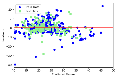
# 学習用、検証用それぞれで残差をプロット
plt.scatter(y_train_pred, y_train_pred - y_train, c = 'blue', marker = 'o', label = 'Train Data')
plt.scatter(y_test_pred, y_test_pred - y_test, c = 'lightgreen', marker = 's', label = 'Test Data')
plt.xlabel('Predicted Values')
plt.ylabel('Residuals')
# 凡例を左上に表示
plt.legend(loc = 'upper left')
# y = 0に直線を引く
plt.hlines(y = 0, xmin = -10, xmax = 50, lw = 2, color = 'red')
plt.xlim([10, 50])
plt.show()

出力結果は次の通り

# 平均二乗誤差を評価するためのメソッドを呼び出し
from sklearn.metrics import mean_squared_error
# 学習用、検証用データに関して平均二乗誤差を出力
print('MSE Train : %.3f, Test : %.3f' % (mean_squared_error(y_train, y_train_pred), mean_squared_error(y_test, y_test_pred)))
# 学習用、検証用データに関してR^2を出力
print('R^2 Train : %.3f, Test : %.3f' % (model.score(X_train, y_train), model.score(X_test, y_test)))

出力結果は次の通り

MSE Train : 44.983, Test : 40.412
R^2 Train : 0.500, Test : 0.434

第２章　非線形回帰モデル

2.1 基底展開法

非線形の場合は、基底展開法を使ってモデリングする
　回帰関数として、基底関数と呼ばれる既知の非線形関数とパラメータベクトルの線形結合を利用する
　未知パラメータについては、最小二乗法もしくは最尤法により推定する
　基底展開法も線形回帰と同じ枠組みで推定可能である

$$y_k=f(x_k)+\epsilon_k \qquad y_i=w_0+\sum_{k=1}^m w_k\phi_k(x_k)+\epsilon_k$$

基底関数の例
多項式関数
$$\phi_k(x)=x^k$$

ガウス型基底関数

$$\phi_k(x)=\exp \Bigg(\frac{(x-\mu_k)^2}{2h_k}\Bigg)$$

スプライン関数

2.2 モデルの式

基底展開法も線形回帰と同じ考え方で推定が可能である。

説明変数（$x\in\mathbb{R^m}$）

$$x_k=(x_{k1},x_{k2},x_{k3},\cdots,x_{km})\in\mathbb{R^m}$$

非線形ベクトル
$$\phi(x_i)=\Big(\phi_1(x_i),\phi_2(x_i),\phi_3(x_i),\cdots ,\phi_k(x_i) \Big)^T\in\mathbb{R^k}$$

非線形関数の計画行列
$$\Phi^{(train)}=\Big(\phi(x_1),\phi(x_2),\phi(x_3),\cdots ,\phi(x_n) \Big)^T\in\mathbb{R^{n\times k}}$$

最尤法による予測
最小二乗法と同様に $\hat{y}$ を求めることができる。
$$\hat{y}=\Phi\Big(\Phi^{(train)T}\Phi^{(train)}\Big)^{-1}\Phi^{(train)T}\Phi^{(train)}$$

2.2 未学習・過学習

機械学習では、データを

１．学習データ
２．検証データ

に分けるのが一般的です。学習データと訓練データに分ける理由は、次に紹介する過学習（Overfitting）を起こさないことが主です。

2.2.1 未学習（Underfitting）

学習データに対して、十分小さな誤差が得られないモデル。つまり、うまく学習できていない
対策　モデルの表現力が低いため、表現力の高いモデルを使用する。特徴量を増やす。

2.2.2 過学習（Overfitting）

学習データに対して誤差は小さくなったものの、検証データに対する誤差が大きいモデル。
つまり、学習データの影響を受けすぎている場合です。

対策
１．学習データを増やす
２．不要な基底関数(説明変数)を削除して、表現力を抑える
３．正則化を使用して表現力を抑える

2.3 正則化（罰則化法）

モデルの複雑さに伴って値が大きくなる正則化項を課した関数を最小化
ただしMSE（）等が最小となる点を探そうとすると過学習を起こす可能性がある。
そのため、原点近辺に制約を与えた上で最小となる点を探す。

$$S_{\gamma}=(y-\Phi^{n \times k}w)^T(y-\Phi w)+\gamma R(w)$$

2.4 L1ノルム、L2ノルム

$L^1$ノルムを利用した時の推定量をラッソ（Lasso）推定量という

$$ R(w)=\sum_{k=1}^m|w_k|=|w_1|+|w_2|+|w_3|+\cdots +|w_m|$$

$L^2$ノルムを利用した時の推定量をリッジ（Ridge）推定量もしくはスパース推定という

$$R(w)=\sqrt{\sum_{k=1}^m w_k^2}=\sqrt{w_1^2+w_2^2+w_3^2+\cdots +w_m^2}$$

2.5 モデルの検証（ホールドアウト法・交差検証）

2.5.1 ホールドアウト法

データを学習用とテスト用の2つに分割する。（学習用データ：テスト用データ＝7:3で分けるなど）
予測精度および誤り率を推定するために使用
デメリットは、手元に大量にデータがない場合、良い性能評価を与えない
基底展開法に基づく非線形回帰モデルでは、基底関数の数、位置、チューニングをホールドアウト値を小さくするモデルで決定する

2.5.2 交差検証（クロスバリデーション）

データをブロックに分割し、1つのブロックを検証用データ、他を学習データとする。
これをイテレーターという。分割した数だけイテレータを繰り返してモデルをそれぞれ作成
できたモデルに対してそれぞれテストデータを与え、得られた精度の平均（CV値）をそれぞれ算出する。
各モデルのうち、最もCV値が小さいものが一番性能が良い

第２章　非線形回帰のハンズオン

モジュールのインポートとseabornの設定

import numpy as np
import matplotlib.pyplot as plt
import seaborn as sns

%matplotlib inline

#seaborn設定
sns.set()
#背景変更
sns.set_style("darkgrid", {'grid.linestyle': '--'})
#大きさ(スケール変更)
sns.set_context("paper")

n=100

def true_func(x):
    z = 1-48*x+218*x**2-315*x**3+145*x**4
    return z 

def linear_func(x):
    z = x
    return z

# 真の関数表示

x = np.arange(0, 1, 0.01)
y = true_func(x)

plt.plot(x, y)
plt.show()

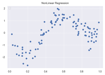
# 真の関数からデータ生成
data = np.random.rand(n).astype(np.float32)
data = np.sort(data)
target = true_func(data)

# ノイズを加える
noise = 0.5 * np.random.randn(n)
target = target + noise

# ノイズ付きデータを描画
plt.scatter(data, target)

plt.title('NonLinear Regression')
plt.legend(loc=2)

from sklearn.linear_model import LinearRegression

clf = LinearRegression()
data = data.reshape(-1, 1)
target = target.reshape(-1, 1)
clf.fit(data, target)

p_lin = clf.predict(data)

plt.scatter(data, target, label='data')
plt.plot(data, p_lin, color='darkorange', marker='', linestyle='-', linewidth=1, markersize=6, label='linear regression')
plt.legend()
print(clf.score(data, target))

0.37878360977970466

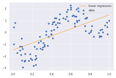
約0.38 と線形回帰ではうまく予測できていないことが分かります。

再度挑戦したところ、

0.19402766475720878

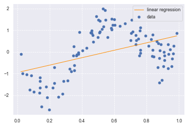
約0.19 と線形回帰ではうまく予測できていないことが分かります。

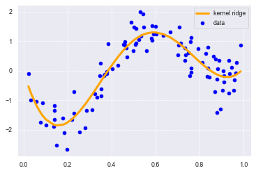
非線形回帰による分析

from sklearn.kernel_ridge import KernelRidge

clf = KernelRidge(alpha=0.0002, kernel='rbf')
clf.fit(data, target)

p_kridge = clf.predict(data)

plt.scatter(data, target, color='blue', label='data')

plt.plot(data, p_kridge, color='orange', linestyle='-', linewidth=3, markersize=6, label='kernel ridge')
plt.legend()

print(clf.score(data, target))

0.8546032766354164

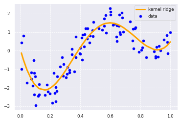
精度が1に近づいている。線形回帰（0.37878360977970466）よりも精度がかなり向上していることがわかります。再度チャレンジしたところ

0.83065477947335

やはり精度が1に近づいています。

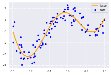
ラッソ回帰の場合は

from sklearn.metrics.pairwise import rbf_kernel
from sklearn.linear_model import Lasso

kx = rbf_kernel(X=data, Y=data, gamma=4)

lasso_clf = Lasso(alpha=0.0001, max_iter=1000)
lasso_clf.fit(kx, target)

p_lasso = lasso_clf.predict(kx)

plt.scatter(data, target, color='blue', label='data')

plt.plot(data, p_lasso, color='orange', linestyle='-', linewidth=3, markersize=3,label='lasso')
plt.legend()

print(lasso_clf.score(kx, target))

0.8494137416910993

リッジ回帰の過学習

#リッジ過学習
from sklearn.kernel_ridge import KernelRidge

#正規化を行わない
clf = KernelRidge(alpha=0.0000,kernel='rbf')
clf.fit(data, target)

p_kridge = clf.predict(data)

plt.scatter(data, target, color='blue', label='data')

plt.plot(data, p_kridge, color='orange', linestyle='-', linewidth=3, markersize=6, label='kernel ridge')
plt.legend()
print(clf.score(data, target))

0.9999999999999979

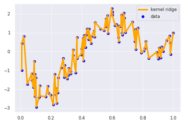
数字は「だけ」いい

scikit-learnのKernelRidgeを利用しない

rbf_kernel：RBFカーネル関数
Ridge：リッジ回帰モデル

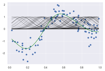
#Ridge
from sklearn.metrics.pairwise import rbf_kernel
from sklearn.linear_model import Ridge

kx = rbf_kernel(X=data, Y=data, gamma=50)

clf = Ridge(alpha=30)
clf.fit(kx, target)

p_ridge = clf.predict(kx)

plt.scatter(data, target,label='data')
for i in range(len(kx)):
    plt.plot(data, kx[i], color='black', linestyle='-', linewidth=1, markersize=3, label='rbf', alpha=0.2)

plt.plot(data, p_ridge, color='green', linestyle='-', linewidth=1, markersize=3,label='ridge regression')

print(clf.score(kx, target))

0.8355822156212662

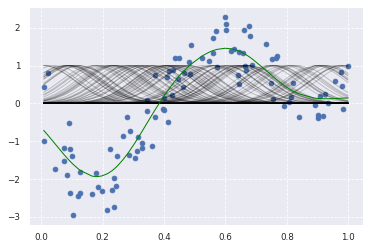
２度目

0.8182710804590342

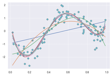
多項式を基底関数とした非線形回帰モデル

1次式から10次式までの多項式をそれぞれ基底関数にした非線形回帰モデル

from sklearn.preprocessing import PolynomialFeatures
from sklearn.pipeline import Pipeline

deg = [1, 2, 3, 4, 5, 6, 7, 8, 9, 10]

for d in deg:
    regr = Pipeline([
        ('poly', PolynomialFeatures(degree=d)),
        ('linear', LinearRegression())
    ])
    regr.fit(data, target)

    # make predictions
    p_poly = regr.predict(data)

    # plot regression result
    plt.scatter(data, target, label='data')
    plt.plot(data, p_poly, label='polynomial of degree %d' % (d))
    print(regr.score(data, target))

出力結果は次の通り

0.37878361384149006
0.5247287010587878
0.6566958180318789
0.857521201080545
0.8596743380417626
0.8598373812208518
0.8602155674528944
0.8615757809921557
0.8616076647596161
0.861566726847494

２度目

0.19402767615562078
0.5517231588121143
0.6211594578122404
0.8339868076733876
0.8372181758831069
0.8377105753616771
0.841044264532349
0.846253471732493
0.846578547945985
0.8462776660848432

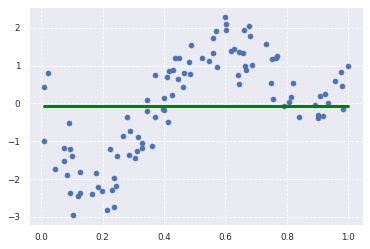
カーネル回帰にラッソ推定量を適用したモデル

rbf_kernel：RBFカーネル関数
Lasso：ラッソ回帰モデル

from sklearn.metrics.pairwise import rbf_kernel
from sklearn.linear_model import Lasso

kx = rbf_kernel(X=data, Y=data, gamma=5)

lasso_clf = Lasso(alpha=10000, max_iter=1000)
lasso_clf.fit(kx, target)

p_lasso = lasso_clf.predict(kx)

plt.scatter(data, target)

plt.plot(data, p_lasso, color='green', linestyle='-', linewidth=3, markersize=3)

print(lasso_clf.score(kx, target))

出力結果は次の通り

-2.220446049250313e-16

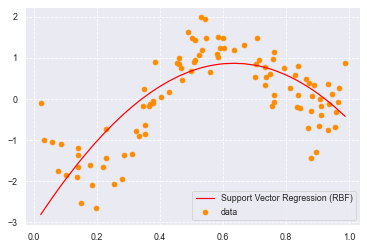
サポートベクター回帰モデル(SVR)

from sklearn import model_selection, preprocessing, linear_model, svm

# SVR-rbf
clf_svr = svm.SVR(kernel='rbf', C=1e3, gamma=0.1, epsilon=0.1)
clf_svr.fit(data, target)
y_rbf = clf_svr.fit(data, target).predict(data)

print(clf_svr.score(data, target))

# plot
plt.scatter(data, target, color='blue', label='data')
plt.plot(data, y_rbf, color='orange', label='Support Vector Regression (RBF)')
plt.legend()
plt.show()

0.5049601396308219

２度目

0.5539489247604701

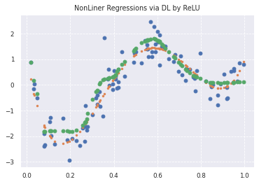
Kerasによる深層学習実装

from sklearn.model_selection import train_test_split
x_train, x_test, y_train, y_test = train_test_split(data, target, test_size=0.1, random_state=0)

from keras.callbacks import EarlyStopping, TensorBoard, ModelCheckpoint

cb_cp = ModelCheckpoint('/content/drive/My Drive/study_ai_ml/skl_ml/out/checkpoints/weights.{epoch:02d}-{val_loss:.2f}.hdf5', verbose=1, save_weights_only=True)
cb_tf  = TensorBoard(log_dir='/content/drive/My Drive/study_ai_ml/skl_ml/out/tensorBoard', histogram_freq=0)

def relu_reg_model():
    model = Sequential()
    model.add(Dense(10, input_dim=1, activation='relu'))
    model.add(Dense(1000, activation='relu'))
    model.add(Dense(1000, activation='relu'))
    model.add(Dense(1000, activation='relu'))
    model.add(Dense(1000, activation='relu'))
    model.add(Dense(1000, activation='relu'))
    model.add(Dense(1000, activation='relu'))
    model.add(Dense(1000, activation='relu'))
    model.add(Dense(1000, activation='linear'))
#     model.add(Dense(100, activation='relu'))
#     model.add(Dense(100, activation='relu'))
#     model.add(Dense(100, activation='relu'))
#     model.add(Dense(100, activation='relu'))
    model.add(Dense(1))

    model.compile(loss='mean_squared_error', optimizer='adam')
    return model

from keras.models import Sequential
from keras.layers import Input, Dense, Dropout, BatchNormalization
from keras.wrappers.scikit_learn import KerasRegressor

# use data split and fit to run the model
estimator = KerasRegressor(build_fn=relu_reg_model, epochs=100, batch_size=5, verbose=1)

history = estimator.fit(x_train, y_train, callbacks=[cb_cp, cb_tf], validation_data=(x_test, y_test))

Epoch 1/100
18/18 [==============================] - 3s 39ms/step - loss: 2.3687 - val_loss: 1.3184

Epoch 00001: saving model to /content/drive/My Drive/study_ai_ml/skl_ml/out/checkpoints/weights.01-1.32.hdf5
Epoch 2/100
18/18 [==============================] - 0s 5ms/step - loss: 1.2527 - val_loss: 0.8765

Epoch 00002: saving model to /content/drive/My Drive/study_ai_ml/skl_ml/out/checkpoints/weights.02-0.88.hdf5
Epoch 3/100
18/18 [==============================] - 0s 5ms/step - loss: 1.3513 - val_loss: 1.1190

Epoch 00003: saving model to /content/drive/My Drive/study_ai_ml/skl_ml/out/checkpoints/weights.03-1.12.hdf5
Epoch 4/100
18/18 [==============================] - 0s 5ms/step - loss: 1.4372 - val_loss: 0.9950

Epoch 00004: saving model to /content/drive/My Drive/study_ai_ml/skl_ml/out/checkpoints/weights.04-1.00.hdf5
Epoch 5/100
18/18 [==============================] - 0s 8ms/step - loss: 1.1755 - val_loss: 0.6253

Epoch 00005: saving model to /content/drive/My Drive/study_ai_ml/skl_ml/out/checkpoints/weights.05-0.63.hdf5
Epoch 6/100
18/18 [==============================] - 0s 6ms/step - loss: 1.0516 - val_loss: 1.0208

Epoch 00006: saving model to /content/drive/My Drive/study_ai_ml/skl_ml/out/checkpoints/weights.06-1.02.hdf5
Epoch 7/100
18/18 [==============================] - 0s 6ms/step - loss: 1.2518 - val_loss: 0.6161

Epoch 00007: saving model to /content/drive/My Drive/study_ai_ml/skl_ml/out/checkpoints/weights.07-0.62.hdf5
Epoch 8/100
18/18 [==============================] - 0s 5ms/step - loss: 1.0415 - val_loss: 0.8969

Epoch 00008: saving model to /content/drive/My Drive/study_ai_ml/skl_ml/out/checkpoints/weights.08-0.90.hdf5
Epoch 9/100
18/18 [==============================] - 0s 5ms/step - loss: 1.0551 - val_loss: 0.6596

Epoch 00009: saving model to /content/drive/My Drive/study_ai_ml/skl_ml/out/checkpoints/weights.09-0.66.hdf5
Epoch 10/100
18/18 [==============================] - 0s 5ms/step - loss: 0.8400 - val_loss: 1.0283

Epoch 00010: saving model to /content/drive/My Drive/study_ai_ml/skl_ml/out/checkpoints/weights.10-1.03.hdf5
Epoch 11/100
18/18 [==============================] - 0s 5ms/step - loss: 1.2764 - val_loss: 0.5673

Epoch 00011: saving model to /content/drive/My Drive/study_ai_ml/skl_ml/out/checkpoints/weights.11-0.57.hdf5
Epoch 12/100
18/18 [==============================] - 0s 7ms/step - loss: 0.7415 - val_loss: 0.6156

Epoch 00012: saving model to /content/drive/My Drive/study_ai_ml/skl_ml/out/checkpoints/weights.12-0.62.hdf5
Epoch 13/100
18/18 [==============================] - 0s 6ms/step - loss: 0.6729 - val_loss: 0.5275

Epoch 00013: saving model to /content/drive/My Drive/study_ai_ml/skl_ml/out/checkpoints/weights.13-0.53.hdf5
Epoch 14/100
18/18 [==============================] - 0s 11ms/step - loss: 0.8777 - val_loss: 0.5321

Epoch 00014: saving model to /content/drive/My Drive/study_ai_ml/skl_ml/out/checkpoints/weights.14-0.53.hdf5
Epoch 15/100
18/18 [==============================] - 0s 5ms/step - loss: 0.8296 - val_loss: 0.6560

Epoch 00015: saving model to /content/drive/My Drive/study_ai_ml/skl_ml/out/checkpoints/weights.15-0.66.hdf5
Epoch 16/100
18/18 [==============================] - 0s 8ms/step - loss: 0.6910 - val_loss: 0.2104

Epoch 00016: saving model to /content/drive/My Drive/study_ai_ml/skl_ml/out/checkpoints/weights.16-0.21.hdf5
Epoch 17/100
18/18 [==============================] - 0s 5ms/step - loss: 0.4999 - val_loss: 0.1959

Epoch 00017: saving model to /content/drive/My Drive/study_ai_ml/skl_ml/out/checkpoints/weights.17-0.20.hdf5
Epoch 18/100
18/18 [==============================] - 0s 5ms/step - loss: 0.4434 - val_loss: 0.1674

Epoch 00018: saving model to /content/drive/My Drive/study_ai_ml/skl_ml/out/checkpoints/weights.18-0.17.hdf5
Epoch 19/100
18/18 [==============================] - 0s 5ms/step - loss: 0.5439 - val_loss: 0.2865

Epoch 00019: saving model to /content/drive/My Drive/study_ai_ml/skl_ml/out/checkpoints/weights.19-0.29.hdf5
Epoch 20/100
18/18 [==============================] - 0s 6ms/step - loss: 0.3424 - val_loss: 0.1589

Epoch 00020: saving model to /content/drive/My Drive/study_ai_ml/skl_ml/out/checkpoints/weights.20-0.16.hdf5
Epoch 21/100
18/18 [==============================] - 0s 6ms/step - loss: 0.4706 - val_loss: 0.1520

Epoch 00021: saving model to /content/drive/My Drive/study_ai_ml/skl_ml/out/checkpoints/weights.21-0.15.hdf5
Epoch 22/100
18/18 [==============================] - 0s 6ms/step - loss: 0.3670 - val_loss: 0.2082

Epoch 00022: saving model to /content/drive/My Drive/study_ai_ml/skl_ml/out/checkpoints/weights.22-0.21.hdf5
Epoch 23/100
18/18 [==============================] - 0s 5ms/step - loss: 0.3142 - val_loss: 0.1180

Epoch 00023: saving model to /content/drive/My Drive/study_ai_ml/skl_ml/out/checkpoints/weights.23-0.12.hdf5
Epoch 24/100
18/18 [==============================] - 0s 5ms/step - loss: 0.3173 - val_loss: 0.2538

Epoch 00024: saving model to /content/drive/My Drive/study_ai_ml/skl_ml/out/checkpoints/weights.24-0.25.hdf5
Epoch 25/100
18/18 [==============================] - 0s 5ms/step - loss: 0.3298 - val_loss: 0.4576

Epoch 00025: saving model to /content/drive/My Drive/study_ai_ml/skl_ml/out/checkpoints/weights.25-0.46.hdf5
Epoch 26/100
18/18 [==============================] - 0s 7ms/step - loss: 0.4976 - val_loss: 0.2659

Epoch 00026: saving model to /content/drive/My Drive/study_ai_ml/skl_ml/out/checkpoints/weights.26-0.27.hdf5
Epoch 27/100
18/18 [==============================] - 0s 5ms/step - loss: 0.4850 - val_loss: 0.3054

Epoch 00027: saving model to /content/drive/My Drive/study_ai_ml/skl_ml/out/checkpoints/weights.27-0.31.hdf5
Epoch 28/100
18/18 [==============================] - 0s 6ms/step - loss: 0.4312 - val_loss: 0.1528

Epoch 00028: saving model to /content/drive/My Drive/study_ai_ml/skl_ml/out/checkpoints/weights.28-0.15.hdf5
Epoch 29/100
18/18 [==============================] - 0s 12ms/step - loss: 0.3060 - val_loss: 0.2119

Epoch 00029: saving model to /content/drive/My Drive/study_ai_ml/skl_ml/out/checkpoints/weights.29-0.21.hdf5
Epoch 30/100
18/18 [==============================] - 0s 11ms/step - loss: 0.3605 - val_loss: 0.2328

Epoch 00030: saving model to /content/drive/My Drive/study_ai_ml/skl_ml/out/checkpoints/weights.30-0.23.hdf5
Epoch 31/100
18/18 [==============================] - 0s 9ms/step - loss: 0.3202 - val_loss: 0.1851

Epoch 00031: saving model to /content/drive/My Drive/study_ai_ml/skl_ml/out/checkpoints/weights.31-0.19.hdf5
Epoch 32/100
18/18 [==============================] - 0s 8ms/step - loss: 0.3274 - val_loss: 0.3435

Epoch 00032: saving model to /content/drive/My Drive/study_ai_ml/skl_ml/out/checkpoints/weights.32-0.34.hdf5
Epoch 33/100
18/18 [==============================] - 0s 6ms/step - loss: 0.3498 - val_loss: 0.3050

Epoch 00033: saving model to /content/drive/My Drive/study_ai_ml/skl_ml/out/checkpoints/weights.33-0.31.hdf5
Epoch 34/100
18/18 [==============================] - 0s 7ms/step - loss: 0.4392 - val_loss: 0.1888

Epoch 00034: saving model to /content/drive/My Drive/study_ai_ml/skl_ml/out/checkpoints/weights.34-0.19.hdf5
Epoch 35/100
18/18 [==============================] - 0s 12ms/step - loss: 0.2745 - val_loss: 0.2376

Epoch 00035: saving model to /content/drive/My Drive/study_ai_ml/skl_ml/out/checkpoints/weights.35-0.24.hdf5
Epoch 36/100
18/18 [==============================] - 0s 11ms/step - loss: 0.3910 - val_loss: 0.1773

Epoch 00036: saving model to /content/drive/My Drive/study_ai_ml/skl_ml/out/checkpoints/weights.36-0.18.hdf5
Epoch 37/100
18/18 [==============================] - 0s 14ms/step - loss: 0.2674 - val_loss: 0.2316

Epoch 00037: saving model to /content/drive/My Drive/study_ai_ml/skl_ml/out/checkpoints/weights.37-0.23.hdf5
Epoch 38/100
18/18 [==============================] - 0s 12ms/step - loss: 0.4182 - val_loss: 0.1392

Epoch 00038: saving model to /content/drive/My Drive/study_ai_ml/skl_ml/out/checkpoints/weights.38-0.14.hdf5
Epoch 39/100
18/18 [==============================] - 0s 13ms/step - loss: 0.2366 - val_loss: 0.1962

Epoch 00039: saving model to /content/drive/My Drive/study_ai_ml/skl_ml/out/checkpoints/weights.39-0.20.hdf5
Epoch 40/100
18/18 [==============================] - 0s 11ms/step - loss: 0.3074 - val_loss: 0.2793

Epoch 00040: saving model to /content/drive/My Drive/study_ai_ml/skl_ml/out/checkpoints/weights.40-0.28.hdf5
Epoch 41/100
18/18 [==============================] - 0s 10ms/step - loss: 0.4282 - val_loss: 0.2520

Epoch 00041: saving model to /content/drive/My Drive/study_ai_ml/skl_ml/out/checkpoints/weights.41-0.25.hdf5
Epoch 42/100
18/18 [==============================] - 0s 9ms/step - loss: 0.3577 - val_loss: 0.2010

Epoch 00042: saving model to /content/drive/My Drive/study_ai_ml/skl_ml/out/checkpoints/weights.42-0.20.hdf5
Epoch 43/100
18/18 [==============================] - 0s 6ms/step - loss: 0.3206 - val_loss: 0.1439

Epoch 00043: saving model to /content/drive/My Drive/study_ai_ml/skl_ml/out/checkpoints/weights.43-0.14.hdf5
Epoch 44/100
18/18 [==============================] - 0s 10ms/step - loss: 0.2555 - val_loss: 0.1906

Epoch 00044: saving model to /content/drive/My Drive/study_ai_ml/skl_ml/out/checkpoints/weights.44-0.19.hdf5
Epoch 45/100
18/18 [==============================] - 0s 11ms/step - loss: 0.3127 - val_loss: 0.2133

Epoch 00045: saving model to /content/drive/My Drive/study_ai_ml/skl_ml/out/checkpoints/weights.45-0.21.hdf5
Epoch 46/100
18/18 [==============================] - 0s 13ms/step - loss: 0.2234 - val_loss: 0.2968

Epoch 00046: saving model to /content/drive/My Drive/study_ai_ml/skl_ml/out/checkpoints/weights.46-0.30.hdf5
Epoch 47/100
18/18 [==============================] - 0s 7ms/step - loss: 0.3244 - val_loss: 0.1655

Epoch 00047: saving model to /content/drive/My Drive/study_ai_ml/skl_ml/out/checkpoints/weights.47-0.17.hdf5
Epoch 48/100
18/18 [==============================] - 0s 8ms/step - loss: 0.3943 - val_loss: 0.1154

Epoch 00048: saving model to /content/drive/My Drive/study_ai_ml/skl_ml/out/checkpoints/weights.48-0.12.hdf5
Epoch 49/100
18/18 [==============================] - 0s 10ms/step - loss: 0.3033 - val_loss: 0.1479

Epoch 00049: saving model to /content/drive/My Drive/study_ai_ml/skl_ml/out/checkpoints/weights.49-0.15.hdf5
Epoch 50/100
18/18 [==============================] - 0s 11ms/step - loss: 0.2892 - val_loss: 0.1643

Epoch 00050: saving model to /content/drive/My Drive/study_ai_ml/skl_ml/out/checkpoints/weights.50-0.16.hdf5
Epoch 51/100
18/18 [==============================] - 0s 11ms/step - loss: 0.3575 - val_loss: 0.1322

Epoch 00051: saving model to /content/drive/My Drive/study_ai_ml/skl_ml/out/checkpoints/weights.51-0.13.hdf5
Epoch 52/100
18/18 [==============================] - 0s 11ms/step - loss: 0.1997 - val_loss: 0.1382

Epoch 00052: saving model to /content/drive/My Drive/study_ai_ml/skl_ml/out/checkpoints/weights.52-0.14.hdf5
Epoch 53/100
18/18 [==============================] - 0s 8ms/step - loss: 0.2448 - val_loss: 0.1006

Epoch 00053: saving model to /content/drive/My Drive/study_ai_ml/skl_ml/out/checkpoints/weights.53-0.10.hdf5
Epoch 54/100
18/18 [==============================] - 0s 7ms/step - loss: 0.3163 - val_loss: 0.2483

Epoch 00054: saving model to /content/drive/My Drive/study_ai_ml/skl_ml/out/checkpoints/weights.54-0.25.hdf5
Epoch 55/100
18/18 [==============================] - 0s 5ms/step - loss: 0.2589 - val_loss: 0.2009

Epoch 00055: saving model to /content/drive/My Drive/study_ai_ml/skl_ml/out/checkpoints/weights.55-0.20.hdf5
Epoch 56/100
18/18 [==============================] - 0s 9ms/step - loss: 0.2954 - val_loss: 0.1127

Epoch 00056: saving model to /content/drive/My Drive/study_ai_ml/skl_ml/out/checkpoints/weights.56-0.11.hdf5
Epoch 57/100
18/18 [==============================] - 0s 9ms/step - loss: 0.2948 - val_loss: 0.2259

Epoch 00057: saving model to /content/drive/My Drive/study_ai_ml/skl_ml/out/checkpoints/weights.57-0.23.hdf5
Epoch 58/100
18/18 [==============================] - 0s 6ms/step - loss: 0.2602 - val_loss: 0.1211

Epoch 00058: saving model to /content/drive/My Drive/study_ai_ml/skl_ml/out/checkpoints/weights.58-0.12.hdf5
Epoch 59/100
18/18 [==============================] - 0s 6ms/step - loss: 0.2215 - val_loss: 0.2863

Epoch 00059: saving model to /content/drive/My Drive/study_ai_ml/skl_ml/out/checkpoints/weights.59-0.29.hdf5
Epoch 60/100
18/18 [==============================] - 0s 5ms/step - loss: 0.1998 - val_loss: 0.1559

Epoch 00060: saving model to /content/drive/My Drive/study_ai_ml/skl_ml/out/checkpoints/weights.60-0.16.hdf5
Epoch 61/100
18/18 [==============================] - 0s 8ms/step - loss: 0.2701 - val_loss: 0.1486

Epoch 00061: saving model to /content/drive/My Drive/study_ai_ml/skl_ml/out/checkpoints/weights.61-0.15.hdf5
Epoch 62/100
18/18 [==============================] - 0s 10ms/step - loss: 0.3268 - val_loss: 0.2724

Epoch 00062: saving model to /content/drive/My Drive/study_ai_ml/skl_ml/out/checkpoints/weights.62-0.27.hdf5
Epoch 63/100
18/18 [==============================] - 0s 7ms/step - loss: 0.3950 - val_loss: 0.2788

Epoch 00063: saving model to /content/drive/My Drive/study_ai_ml/skl_ml/out/checkpoints/weights.63-0.28.hdf5
Epoch 64/100
18/18 [==============================] - 0s 5ms/step - loss: 0.4328 - val_loss: 0.1337

Epoch 00064: saving model to /content/drive/My Drive/study_ai_ml/skl_ml/out/checkpoints/weights.64-0.13.hdf5
Epoch 65/100
18/18 [==============================] - 0s 6ms/step - loss: 0.3054 - val_loss: 0.1788

Epoch 00065: saving model to /content/drive/My Drive/study_ai_ml/skl_ml/out/checkpoints/weights.65-0.18.hdf5
Epoch 66/100
18/18 [==============================] - 0s 5ms/step - loss: 0.2838 - val_loss: 0.1487

Epoch 00066: saving model to /content/drive/My Drive/study_ai_ml/skl_ml/out/checkpoints/weights.66-0.15.hdf5
Epoch 67/100
18/18 [==============================] - 0s 9ms/step - loss: 0.2816 - val_loss: 0.2568

Epoch 00067: saving model to /content/drive/My Drive/study_ai_ml/skl_ml/out/checkpoints/weights.67-0.26.hdf5
Epoch 68/100
18/18 [==============================] - 0s 10ms/step - loss: 0.3562 - val_loss: 0.2701

Epoch 00068: saving model to /content/drive/My Drive/study_ai_ml/skl_ml/out/checkpoints/weights.68-0.27.hdf5
Epoch 69/100
18/18 [==============================] - 0s 5ms/step - loss: 0.4052 - val_loss: 0.1701

Epoch 00069: saving model to /content/drive/My Drive/study_ai_ml/skl_ml/out/checkpoints/weights.69-0.17.hdf5
Epoch 70/100
18/18 [==============================] - 0s 14ms/step - loss: 0.2667 - val_loss: 0.2477

Epoch 00070: saving model to /content/drive/My Drive/study_ai_ml/skl_ml/out/checkpoints/weights.70-0.25.hdf5
Epoch 71/100
18/18 [==============================] - 0s 11ms/step - loss: 0.2383 - val_loss: 0.1706

Epoch 00071: saving model to /content/drive/My Drive/study_ai_ml/skl_ml/out/checkpoints/weights.71-0.17.hdf5
Epoch 72/100
18/18 [==============================] - 0s 10ms/step - loss: 0.3184 - val_loss: 0.1495

Epoch 00072: saving model to /content/drive/My Drive/study_ai_ml/skl_ml/out/checkpoints/weights.72-0.15.hdf5
Epoch 73/100
18/18 [==============================] - 0s 8ms/step - loss: 0.3163 - val_loss: 0.3475

Epoch 00073: saving model to /content/drive/My Drive/study_ai_ml/skl_ml/out/checkpoints/weights.73-0.35.hdf5
Epoch 74/100
18/18 [==============================] - 0s 8ms/step - loss: 0.3339 - val_loss: 0.1130

Epoch 00074: saving model to /content/drive/My Drive/study_ai_ml/skl_ml/out/checkpoints/weights.74-0.11.hdf5
Epoch 75/100
18/18 [==============================] - 0s 6ms/step - loss: 0.2950 - val_loss: 0.1577

Epoch 00075: saving model to /content/drive/My Drive/study_ai_ml/skl_ml/out/checkpoints/weights.75-0.16.hdf5
Epoch 76/100
18/18 [==============================] - 0s 6ms/step - loss: 0.2316 - val_loss: 0.1398

Epoch 00076: saving model to /content/drive/My Drive/study_ai_ml/skl_ml/out/checkpoints/weights.76-0.14.hdf5
Epoch 77/100
18/18 [==============================] - 0s 5ms/step - loss: 0.2111 - val_loss: 0.1690

Epoch 00077: saving model to /content/drive/My Drive/study_ai_ml/skl_ml/out/checkpoints/weights.77-0.17.hdf5
Epoch 78/100
18/18 [==============================] - 0s 6ms/step - loss: 0.3059 - val_loss: 0.2156

Epoch 00078: saving model to /content/drive/My Drive/study_ai_ml/skl_ml/out/checkpoints/weights.78-0.22.hdf5
Epoch 79/100
18/18 [==============================] - 0s 6ms/step - loss: 0.2102 - val_loss: 0.1805

Epoch 00079: saving model to /content/drive/My Drive/study_ai_ml/skl_ml/out/checkpoints/weights.79-0.18.hdf5
Epoch 80/100
18/18 [==============================] - 0s 6ms/step - loss: 0.3325 - val_loss: 0.1725

Epoch 00080: saving model to /content/drive/My Drive/study_ai_ml/skl_ml/out/checkpoints/weights.80-0.17.hdf5
Epoch 81/100
18/18 [==============================] - 0s 6ms/step - loss: 0.2600 - val_loss: 0.2401

Epoch 00081: saving model to /content/drive/My Drive/study_ai_ml/skl_ml/out/checkpoints/weights.81-0.24.hdf5
Epoch 82/100
18/18 [==============================] - 0s 11ms/step - loss: 0.2752 - val_loss: 0.1804

Epoch 00082: saving model to /content/drive/My Drive/study_ai_ml/skl_ml/out/checkpoints/weights.82-0.18.hdf5
Epoch 83/100
18/18 [==============================] - 0s 5ms/step - loss: 0.2183 - val_loss: 0.1633

Epoch 00083: saving model to /content/drive/My Drive/study_ai_ml/skl_ml/out/checkpoints/weights.83-0.16.hdf5
Epoch 84/100
18/18 [==============================] - 0s 6ms/step - loss: 0.3495 - val_loss: 0.1369

Epoch 00084: saving model to /content/drive/My Drive/study_ai_ml/skl_ml/out/checkpoints/weights.84-0.14.hdf5
Epoch 85/100
18/18 [==============================] - 0s 5ms/step - loss: 0.2212 - val_loss: 0.1626

Epoch 00085: saving model to /content/drive/My Drive/study_ai_ml/skl_ml/out/checkpoints/weights.85-0.16.hdf5
Epoch 86/100
18/18 [==============================] - 0s 5ms/step - loss: 0.1862 - val_loss: 0.1461

Epoch 00086: saving model to /content/drive/My Drive/study_ai_ml/skl_ml/out/checkpoints/weights.86-0.15.hdf5
Epoch 87/100
18/18 [==============================] - 0s 5ms/step - loss: 0.1649 - val_loss: 0.1199

Epoch 00087: saving model to /content/drive/My Drive/study_ai_ml/skl_ml/out/checkpoints/weights.87-0.12.hdf5
Epoch 88/100
18/18 [==============================] - 0s 5ms/step - loss: 0.2830 - val_loss: 0.1360

Epoch 00088: saving model to /content/drive/My Drive/study_ai_ml/skl_ml/out/checkpoints/weights.88-0.14.hdf5
Epoch 89/100
18/18 [==============================] - 0s 11ms/step - loss: 0.2637 - val_loss: 0.1703

Epoch 00089: saving model to /content/drive/My Drive/study_ai_ml/skl_ml/out/checkpoints/weights.89-0.17.hdf5
Epoch 90/100
18/18 [==============================] - 0s 16ms/step - loss: 0.2872 - val_loss: 0.1716

Epoch 00090: saving model to /content/drive/My Drive/study_ai_ml/skl_ml/out/checkpoints/weights.90-0.17.hdf5
Epoch 91/100
18/18 [==============================] - 0s 16ms/step - loss: 0.2421 - val_loss: 0.1363

Epoch 00091: saving model to /content/drive/My Drive/study_ai_ml/skl_ml/out/checkpoints/weights.91-0.14.hdf5
Epoch 92/100
18/18 [==============================] - 0s 11ms/step - loss: 0.3171 - val_loss: 0.1216

Epoch 00092: saving model to /content/drive/My Drive/study_ai_ml/skl_ml/out/checkpoints/weights.92-0.12.hdf5
Epoch 93/100
18/18 [==============================] - 0s 10ms/step - loss: 0.3229 - val_loss: 0.1370

Epoch 00093: saving model to /content/drive/My Drive/study_ai_ml/skl_ml/out/checkpoints/weights.93-0.14.hdf5
Epoch 94/100
18/18 [==============================] - 0s 6ms/step - loss: 0.2654 - val_loss: 0.1550

Epoch 00094: saving model to /content/drive/My Drive/study_ai_ml/skl_ml/out/checkpoints/weights.94-0.16.hdf5
Epoch 95/100
18/18 [==============================] - 0s 5ms/step - loss: 0.2720 - val_loss: 0.1576

Epoch 00095: saving model to /content/drive/My Drive/study_ai_ml/skl_ml/out/checkpoints/weights.95-0.16.hdf5
Epoch 96/100
18/18 [==============================] - 0s 5ms/step - loss: 0.2874 - val_loss: 0.1960

Epoch 00096: saving model to /content/drive/My Drive/study_ai_ml/skl_ml/out/checkpoints/weights.96-0.20.hdf5
Epoch 97/100
18/18 [==============================] - 0s 6ms/step - loss: 0.3330 - val_loss: 0.2022

Epoch 00097: saving model to /content/drive/My Drive/study_ai_ml/skl_ml/out/checkpoints/weights.97-0.20.hdf5
Epoch 98/100
18/18 [==============================] - 0s 5ms/step - loss: 0.2197 - val_loss: 0.1240

Epoch 00098: saving model to /content/drive/My Drive/study_ai_ml/skl_ml/out/checkpoints/weights.98-0.12.hdf5
Epoch 99/100
18/18 [==============================] - 0s 5ms/step - loss: 0.2322 - val_loss: 0.1977

Epoch 00099: saving model to /content/drive/My Drive/study_ai_ml/skl_ml/out/checkpoints/weights.99-0.20.hdf5
Epoch 100/100
18/18 [==============================] - 0s 5ms/step - loss: 0.2265 - val_loss: 0.1991

Epoch 00100: saving model to /content/drive/My Drive/study_ai_ml/skl_ml/out/checkpoints/weights.100-0.20.hdf5

y_pred = estimator.predict(x_train)

18/18 [==============================] - 0s 2ms/step

plt.title('NonLiner Regressions via DL by ReLU')
plt.plot(data, target, 'o')
plt.plot(data, true_func(data), '.')
plt.plot(x_train, y_pred, "o", label='predicted: deep learning')
#plt.legend(loc=2)

print(lasso_clf.coef_)

[-0. -0. -0. -0. -0. -0. -0. -0. -0. -0. -0. -0. -0. -0. -0. -0. -0. -0.
-0. -0. -0. -0. -0. -0. -0. -0. -0. -0. -0. -0. -0. -0. -0. -0. -0. -0.
0. 0. 0. 0. 0. 0. 0. 0. 0. 0. 0. 0. 0. 0. 0. 0. 0. 0.
0. 0. 0. 0. 0. 0. 0. 0. 0. 0. 0. 0. 0. 0. 0. 0. 0. 0.
0. 0. 0. 0. 0. 0. 0. 0. 0. 0. 0. 0. 0. 0. 0. 0. 0. 0.
0. 0. 0. 0. 0. 0. 0. 0. 0. 0.]

第３章　ロジスティック回帰モデル

ロジスティック回帰は回帰問題を扱うモデルではなく、分類問題を扱うモデルである。

3.1 分類問題

教師あり学習の1つで、ある入力値からどのクラスに分類するか予測する

3.2 分類で扱うデータ

入力：説明変数
$m$次元のベクトル

$$x=(x_1,x_2,x_3,\cdots,x_m)^T\in\mathbb{R^m}$$
出力：目的変数
離散値$y\in$｛0,1｝

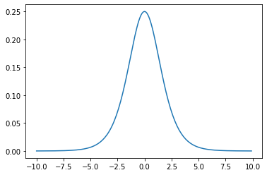
3.3 シグモイド関数

シグモイド関数 $\sigma(x)$ は、入力が実数のとき必ず出力が0と1に収まる単調増加関数

$$\sigma(x)=\frac{1}{1+\exp(-ax)}=\frac{1}{1+e^{-ax}}$$

シグモイド関数の微分はシグモイド関数自身で表現できる。
$$\sigma^{\prime}(x)=a\sigma(x)\big(1-\sigma(x) \big)$$

証明

\begin{eqnarray}
\sigma^{\prime}(x)&=&\bigg(\frac{1}{1+e^{-ax}}\bigg)^{\prime}\\
&=&\frac{-\big(-ae^{-ax}\big)}{(1+e^{-ax})^2}\\
&=&a\times\frac{1}{1+e^{-ax}}\times \frac{e^{-ax}}{1+e^{-ax}}\\
&=&a\times\frac{1}{1+e^{-ax}}\times \bigg(1-\frac{1}{1+e^{-ax}} \bigg)\\
&=&a\sigma (x)\Big(1- \sigma (x)\Big)
\end{eqnarray}

線形結合した値をシグモイド関数に与えることで$y=1$となる確率が出力
$$P(Y=1|x)=\sigma(w_0+w_1x_1+w_2x_2+w_3x_3+\cdots+w_mx_m)$$
出力された確率が0.5以上なら1、未満なら0とする

この数式を考察する際に最尤推定を使用する

3.4 最尤推定

元のデータである$x$、$y$を生成するに至る尤もらしいパラメータを探す推定方法
尤度関数を最大化させる未知のパラメータを探す
ロジスティック回帰モデルではベルヌーイ分布を利用する

3.5 尤度関数

データを固定し、パラメータを変化させる
1回の試行で$y=y_1$となる確率
$$p(y)=p^y(1-p)^{1-y}$$

$n$回の試行で同時に、$y_1,y_2,y_3,\cdots,y_n$が起こる確率

\begin{eqnarray}
P(y_1,y_2,y_3,\cdots,y_n ;p)&=&\prod_{k=1}^np^{y_k}(1-p)^{1-y_k} \\
&=&\prod_{k=1}^n \Big(\sigma(w^Tx_k) \Big)^{y_k}\Big(1-\sigma(w^Tx_k)\Big)^{1-y_k} \\
&=& L(w)
\end{eqnarray}

3.6 対数尤度関数

尤度関数は式が積の形になっているので、対数を取り和の形に直すと計算が楽になる
対数尤度関数が最大になる点と尤度関数が最大になる点は同じとなる。

\begin{eqnarray}
-\log L(w)&=&-\log L(w_1,w_2,w_3,\cdots,w_m)\\
&=&-\Big(y_1\log y_1+\cdots+y_m\log y_m+(1-y_1)\log (1-y_1)+\cdots+ (1-y_m)\log (1-y_m)+\Big)\\
&=&-\sum_{k=1}^m\Big(y_k\log y_k+(1-y_k)\log(1-y_k) \Big)
\end{eqnarray}

対数尤度関数を微分して0になる点を求めることができないため、勾配降下法を使って逐次求める。

3.7 勾配降下法

反復学習でパラメータを逐次更新する方法
パラメータ$k$が更新されなくなったとき、最適解が見つかったことになる。

$$w^{k+1}=w^k-\eta\sum_{i=1}^n(y_i-p_i)x_i$$

データを全て使うため大量のメモリが必要になる。
計算時間が多くなる問題がある。
最適解ではなく局所最適解に収束する可能性がある。

3.8 確率的勾配降下法

データを1件ずつランダムに選び、パラメータを更新する勾配降下法

$$w^{k+1}=w^k-\eta(y_i-p_i)x_i$$

3.9 モデルの評価

3.10 混合行列

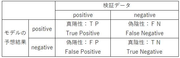
１．真陽性：TP（True Positive）　⇒　正しくPositiveと判別した数
２．偽陽性：FP（False Positive）　⇒　間違えてPositiveと判別した数
３．真陰性：TN（True Negative）　⇒　正しくNegativeと判別した数
４．偽陰性；FN（False Negative）　⇒　間違えてNegativeと判別した数

3.10.1 正解率（Accuracy）

全データ（$TP+FN+FP+TN$）のうち、正しく判別した（$TP+TN$）確率
$$\frac{TP+TN}{TP+FN+FP+TN}$$

3.10.2 再現率（Recall）

Positiveなデータ（$TP+FN$）から、Positiveと予想（$TP$）できる確率
$$\frac{TP}{TP+FN}$$

3.10.3 適合率（Precision）

モデルがPositiveと予想したデータ$TP+FP$から、Positiveと予想（$TP$）できる確率
$$\frac{TP}{TP+FP}=P$$

3.10.4 F値(F score)

再現率（Recall）と適合率（Precision）の調和平均
$$\frac{2}{\frac{1}{Recall}+\frac{1}{Precision}}=\frac{2(Precision)(Recall)}{Recall+Precision}$$

第３章 ロジスティック回帰のハンズオン

モジュールの読み込み・データ表示

#from モジュール名 import クラス名（もしくは関数名や変数名）
import pandas as pd
from pandas import DataFrame
import numpy as np
import matplotlib.pyplot as plt
import seaborn as sns

#matplotlibをinlineで表示するためのおまじない (plt.show()しなくていい)
%matplotlib inline

データの読み込み

# titanic data csvファイルの読み込み
titanic_df = pd.read_csv('../data/titanic_train.csv')

データセットの確認

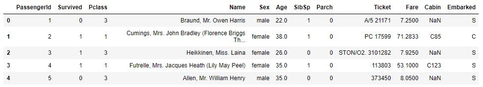
# ファイルの先頭部を表示し、データセットを確認する
titanic_df.head(5)

不要なデータの削除する

#予測に不要と考えるからうをドロップ (本当はここの情報もしっかり使うべきだと思っています)
titanic_df.drop(['PassengerId', 'Name', 'Ticket', 'Cabin'], axis=1, inplace=True)

#一部カラムをドロップしたデータを表示
titanic_df.head()

欠損値の補完をする

#nullを含んでいる行を表示
titanic_df[titanic_df.isnull().any(1)].head(10)

#Ageカラムのnullを中央値で補完

titanic_df['AgeFill'] = titanic_df['Age'].fillna(titanic_df['Age'].mean())

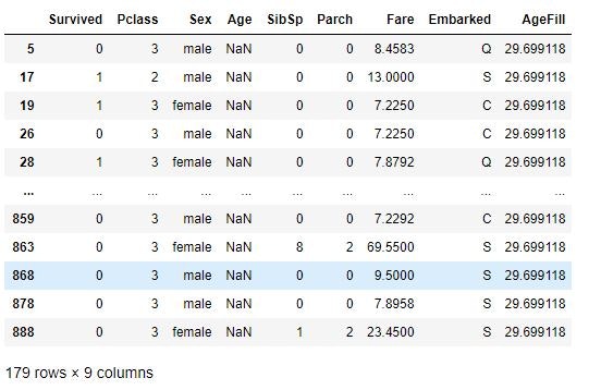
#再度nullを含んでいる行を表示 (Ageのnullは補完されている)
titanic_df[titanic_df.isnull().any(1)]

#titanic_df.dtypes

ロジスティック回帰の実装（チケット価格から生死を判別）

# 運賃だけのリストを作成(説明変数)
data1 = titanic_df.loc[:, ["Fare"]].values

# 生死フラグのみのリストを作成(目的変数)
label1 = titanic_df.loc[:, ["Survived"]].values

from sklearn.linear_model import LogisticRegression

# ロジスティック回帰モデルのインスタンスを生成して学習
model = LogisticRegression()
model.fit(data1, label1)

LogisticRegression()

結果の確認

# model.predict(61)
print(model.predict([[61]]))

#model.predict_proba(62)
print(model.predict([[62]]))

[0]
[1]

X_test_value = model.decision_function(data1) 
print(model.predict([[62]]))
print(model.predict_proba([[62]]))

[[0.50358033 0.49641967]]
[[0.49978123 0.50021877]]

print (model.intercept_)

print (model.coef_)

[-0.94131796]
[[0.01519666]]

w_0 = model.intercept_[0]
w_1 = model.coef_[0,0]

# def normal_sigmoid(x):
#     return 1 / (1+np.exp(-x))

def sigmoid(x):
    return 1 / (1+np.exp(-(w_1*x+w_0)))

x_range = np.linspace(-1, 500, 3000)

plt.figure(figsize=(9,5))
#plt.xkcd()
plt.legend(loc=2)


# plt.ylim(-0.1, 1.1)
# plt.xlim(-10, 10)

# plt.plot([-10,10],[0,0], "k", lw=1)
# plt.plot([0,0],[-1,1.5], "k", lw=1)
plt.plot(data1,np.zeros(len(data1)), 'o')
plt.plot(data1, model.predict_proba(data1), 'o')
plt.plot(x_range, sigmoid(x_range), '-')
#plt.plot(x_range, normal_sigmoid(x_range), '-')
#

ロジスティック回帰の実装（2変数から生死を判別）

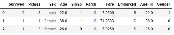
titanic_df['Gender'] = titanic_df['Sex'].map({'female': 0, 'male': 1}).astype(int)
titanic_df.head(3)

性別（sex）が
男性︓male 、 女性︓female
のため、計算ができない。
そこで、男性︓male＝1 、 女性︓female=0とした
変数「Gender」を作成する。

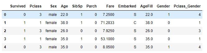
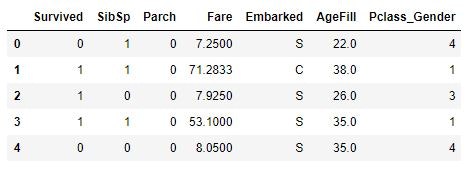
titanic_df['Pclass_Gender'] = titanic_df['Pclass'] + titanic_df['Gender']
titanic_df.head()

Pclass_Gender を　Pclass（乗客の社会階級）＋Gender（乗客の性別）で定義する。
Pclassは、1 が High class / 2 が Middle class / 3 がLow class
Genderは、1 が男性 / 0 が女性

Pclass = 1 ⇒　High classの女性
Pclass = 2 ⇒　High classの男性 or Middle classの女性
Pclass = 3 ⇒　Middle classの男性 or Low classの女性
Pclass = 4 ⇒　Low classの男性 or

titanic_df = titanic_df.drop(['Pclass', 'Sex', 'Gender','Age'], axis=1)
titanic_df.head()

np.random.seed = 0

xmin, xmax = -5, 85
ymin, ymax = 0.5, 4.5

index_survived = titanic_df[titanic_df["Survived"]==0].index
index_notsurvived = titanic_df[titanic_df["Survived"]==1].index

from matplotlib.colors import ListedColormap
fig, ax = plt.subplots()
cm = plt.cm.RdBu
cm_bright = ListedColormap(['#FF0000', '#0000FF'])
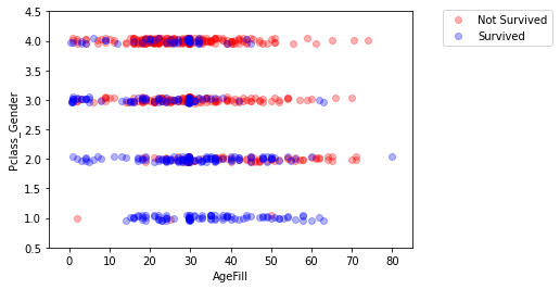
sc = ax.scatter(titanic_df.loc[index_survived, 'AgeFill'],
                titanic_df.loc[index_survived, 'Pclass_Gender']+(np.random.rand(len(index_survived))-0.5)*0.1,
                color='r', label='Not Survived', alpha=0.3)
sc = ax.scatter(titanic_df.loc[index_notsurvived, 'AgeFill'],
                titanic_df.loc[index_notsurvived, 'Pclass_Gender']+(np.random.rand(len(index_notsurvived))-0.5)*0.1,
                color='b', label='Survived', alpha=0.3)
ax.set_xlabel('AgeFill')
ax.set_ylabel('Pclass_Gender')
ax.set_xlim(xmin, xmax)
ax.set_ylim(ymin, ymax)
ax.legend(bbox_to_anchor=(1.4, 1.03))

matplotlib.legend.Legend at 0x1e9027ba730

#運賃だけのリストを作成（説明変数）
data2 = titanic_df.loc[:, ["AgeFill", "Pclass_Gender"]].values
data2

array([[22. , 4. ],
[38. , 1. ],
[26. , 3. ],
...,
[29.69911765, 3. ],
[26. , 2. ],
[32. , 4. ]])

#生死フラグのみのリストを作成（目的変数）
label2 =  titanic_df.loc[:,["Survived"]].values

model2 = LogisticRegression()

model2.fit(data2, label2)

LogisticRegression()

model2.predict([[10,1]])

array([1], dtype=int64)

model2.predict_proba([[10,1]])

array([[0.03754749, 0.96245251]])

10歳でHigh classの女性（Pclass = 1）は96%で生存すると予測

課題：年齢が30歳で男の乗客は生き残れるか
を男性の社会的地位によって場合分けする。

print(model2.predict([[30,2]]))
print(model2.predict_proba([[30, 2]]))

High class ⇒　Pclass = 2　　⇒　model2.predict_proba([[30, 2]])
結果：生存者と予想、生存率69.1%

[1]
[[0.30829809 0.69170191]]

print(model2.predict([[30,3]]))
print(model2.predict_proba([[30, 3]]))

Middle class ⇒　Pclass = 3　⇒　model2.predict_proba([[30, 3]])
結果：死者と予想、生存率33.1%

[0]
[[0.66890121 0.33109879]]

print(model2.predict([[30,4]]))
print(model2.predict_proba([[30, 4]]))

Low class ⇒　Pclass = 4　⇒　model2.predict_proba([[30, 4]])
結果：死者と予想、生存率9.8%

[0]
[[0.90154649 0.09845351]]

h = 0.02
xmin, xmax = -5, 85
ymin, ymax = 0.5, 4.5
xx, yy = np.meshgrid(np.arange(xmin, xmax, h), np.arange(ymin, ymax, h))
Z = model2.predict_proba(np.c_[xx.ravel(), yy.ravel()])[:, 1]
Z = Z.reshape(xx.shape)

fig, ax = plt.subplots()
levels = np.linspace(0, 1.0)
cm = plt.cm.RdBu
cm_bright = ListedColormap(['#FF0000', '#0000FF'])
#contour = ax.contourf(xx, yy, Z, cmap=cm, levels=levels, alpha=0.5)

sc = ax.scatter(titanic_df.loc[index_survived, 'AgeFill'],
                titanic_df.loc[index_survived, 'Pclass_Gender']+(np.random.rand(len(index_survived))-0.5)*0.1,
                color='r', label='Not Survived', alpha=0.3)
sc = ax.scatter(titanic_df.loc[index_notsurvived, 'AgeFill'],
                titanic_df.loc[index_notsurvived, 'Pclass_Gender']+(np.random.rand(len(index_notsurvived))-0.5)*0.1,
                color='b', label='Survived', alpha=0.3)

ax.set_xlabel('AgeFill')
ax.set_ylabel('Pclass_Gender')
ax.set_xlim(xmin, xmax)
ax.set_ylim(ymin, ymax)
#fig.colorbar(contour)

x1 = xmin
x2 = xmax
y1 = -1*(model2.intercept_[0]+model2.coef_[0][0]*xmin)/model2.coef_[0][1]
y2 = -1*(model2.intercept_[0]+model2.coef_[0][0]*xmax)/model2.coef_[0][1]
ax.plot([x1, x2] ,[y1, y2], 'k--')

モデル評価（混同行列とクロスバリデーション）

from sklearn.model_selection import train_test_split

# 1つの説明変数(Fare)のデータ
traindata1, testdata1, trainlabel1, testlabel1 = train_test_split(data1, label1, test_size=0.2)
traindata1.shape
trainlabel1.shape

# 2つの説明変数(AgeFill, Pclass_Gender)のデータ
traindata2, testdata2, trainlabel2, testlabel2 = train_test_split(data2, label2, test_size=0.2)
traindata2.shape
trainlabel2.shape
# 本来は同じデータセットを分割しなければいけない。(簡易的に別々に分割している。)

eval_model1=LogisticRegression()
eval_model2=LogisticRegression()

predictor_eval1=eval_model1.fit(traindata1, trainlabel1).predict(testdata1)
predictor_eval2=eval_model2.fit(traindata2, trainlabel2).predict(testdata2)
#predictor_eval=eval_model.fit(traindata, trainlabel).predict(testdata)

(712, 1)

eval_model1.score(traindata1, trainlabel1)

説明変数が1：学習データの決定係数

0.6685393258426966

eval_model1.score(testdata1,testlabel1)

説明変数が1：検証データの決定係数

0.6703910614525139

eval_model2.score(traindata2, trainlabel2)

説明変数が2：学習データの決定係数

0.7668539325842697

eval_model1.score(testdata1,testlabel1)

説明変数が2：検証データの決定係数

0.8100558659217877

説明変数が2のモデルのほうが、やはり精度が良い。

from sklearn import metrics
print(metrics.classification_report(testlabel1, predictor_eval1))
print(metrics.classification_report(testlabel2, predictor_eval2))

説明変数が1

	precision	recall	f1-score	support
0	0.65	0.99	0.78	107
1	0.93	0.19	0.32	72
accuracy			0.67	179
macro avg	0.79	0.59	0.55	179
weighted avg	0.76	0.67	0.60	179

説明変数が2

	precision	recall	f1-score	support
0	0.85	0.87	0.86	119
1	0.73	0.68	0.71	60
accuracy			0.81	179
macro avg	0.79	0.78	0.78	179
weighted avg	0.81	0.81	0.81	179

混合行列

from sklearn.metrics import confusion_matrix
confusion_matrix1=confusion_matrix(testlabel1, predictor_eval1)
confusion_matrix2=confusion_matrix(testlabel2, predictor_eval2)

confusion_matrix1

array([[106, 1],
[ 58, 14]], dtype=int64)

confusion_matrix2

array([[104, 15],
[ 19, 41]], dtype=int64)

fig = plt.figure(figsize = (7,7))
#plt.title(title)
sns.heatmap(
    confusion_matrix1,
    vmin=None,
    vmax=None,
    cmap="Blues",
    center=None,
    robust=False,
    annot=True, fmt='.2g',
    annot_kws=None,
    linewidths=0,
    linecolor='white',
    cbar=True,
    cbar_kws=None,
    cbar_ax=None,
    square=True, ax=None, 
    #xticklabels=columns,
    #yticklabels=columns,
    mask=None)

fig = plt.figure(figsize = (7,7))
#plt.title(title)
sns.heatmap(
    confusion_matrix2,
    vmin=None,
    vmax=None,
    cmap="Blues",
    center=None,
    robust=False,
    annot=True, fmt='.2g',
    annot_kws=None,
    linewidths=0,
    linecolor='white',
    cbar=True,
    cbar_kws=None,
    cbar_ax=None,
    square=True, ax=None, 
    #xticklabels=columns,
    #yticklabels=columns,
    mask=None)

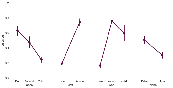
#Paired categorical plots

import seaborn as sns
sns.set(style="whitegrid")

# Load the example Titanic dataset
titanic = sns.load_dataset("titanic")

# Set up a grid to plot survival probability against several variables
g = sns.PairGrid(titanic, y_vars="survived",
                 x_vars=["class", "sex", "who", "alone"],
                 size=5, aspect=.5)

# Draw a seaborn pointplot onto each Axes
g.map(sns.pointplot, color=sns.xkcd_rgb["plum"])
g.set(ylim=(0, 1))
sns.despine(fig=g.fig, left=True)

plt.show()

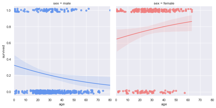
#Faceted logistic regression

import seaborn as sns
sns.set(style="darkgrid")

# Load the example titanic dataset
df = sns.load_dataset("titanic")

# Make a custom palette with gendered colors
pal = dict(male="#6495ED", female="#F08080")

# Show the survival proability as a function of age and sex
g = sns.lmplot(x="age", y="survived", col="sex", hue="sex", data=df,
               palette=pal, y_jitter=.02, logistic=True)
g.set(xlim=(0, 80), ylim=(-.05, 1.05))
plt.show()

第４章　主成分分析

線形変換後の変数の分散が最大となる射影軸を探索することにより、多変量データの持つ構造をより少数個の指標に圧縮する。

学習データ
$$x_i=(x_{i1},x_{i2},x_{i3},\cdots,x_{im})\in\mathbb{R^m}$$

平均（ベクトル）
$$\bar{x}=\frac{1}{n}\sum_{i=1}^n x_i$$

データ行列
$$\bar{X}=\Big(x_1-\bar{x},x_2-\bar{x},x_3-\bar{x},\cdots x_n-\bar{x}, \big)^T$$

分散共分散行列
$$Var(\bar{X})=\frac{1}{n}\bar{X}^T\bar{X} $$

線形変換後のベクトル
$$s_j=(s_{1j},s_{2j},s_{3j},\cdots,s_{nj})^{T}=\bar{X}a_j\qquad a_j\in\mathbb{R^m}$$
$j$ は射影軸のインデックス

4.1 ラグランジュ関数（目的関数・制約条件）

目的関数
$$\arg\max_{a\in\mathbb{R^m}} a_j^T Var(\bar{X}) a_j$$

制約条件は
$$a_j^Ta_j=1$$

制約条件付の最適化問題
⇒　ラグランジュ関数を最大にする係数ベクトル（微分して0になる点）を探索

4.2 ラグランジュ関数

$$E(a_j)=a_j^T Var(\bar{X}) a_j -\lambda \left(a_j^Ta_j-1\right)$$

ラグランジュ関数の両辺を微分して、係数ベクトル（微分して0になる点）を探す
$$\frac{\partial E(a_j)}{\partial a_j}=2Var (\bar{X})a_j-2\lambda a_j \quad (=0)$$
両辺2で割って、移行すると
$$Var (\bar{X})a_j=\lambda a_j$$
射影先の分散は固有値と一致する
$$Var (s_1)=a_1^TVar (\bar{X})a_1 =\lambda_1 a_1^Ta_1=\lambda_1$$

4.3 寄与率

第$k$主成分の分散の全分散に対する割合（第$k$主成分が持つ情報量の割合）のことを寄与率$c_k$という
$$c_k=\frac{\lambda_k}{\displaystyle\sum_{i=1}^m\lambda_i}=\frac{\lambda_k}{\lambda_1+\lambda_2+\lambda_3+\cdots+\lambda_k +\cdots+\lambda_m}$$

4.4 累積寄与率

第1から第$k$主成分まで圧縮した際の情報損失量の割合のことを累積寄与率$r_k$という。
$$c_k=\frac{\displaystyle\sum_{j=1}^k\lambda_j}{\displaystyle\sum_{i=1}^m\lambda_i}=\frac{\lambda_1+\lambda_2+\lambda_3+\cdots+\lambda_k }{\lambda_1+\lambda_2+\lambda_3+\cdots+\lambda_k +\cdots+\lambda_m}$$

乳がん検査データを利用しロジスティック回帰モデルを作成
主成分を利用し2次元空間上に次元圧縮

第４章　ＰＣＡのハンズオン

必要なモジュールのインポート

import pandas as pd
from sklearn.model_selection import train_test_split
from sklearn.preprocessing import StandardScaler
from sklearn.linear_model import LogisticRegressionCV
from sklearn.metrics import confusion_matrix
from sklearn.decomposition import PCA
import matplotlib.pyplot as plt
%matplotlib inline

csvファイルから読み込む。

cancer_df = pd.read_csv('data/cancer.csv')

print('cancer df shape: {}'.format(cancer_df.shape))

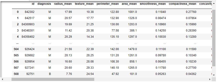
cancer df shape: (569, 33)

569レコード、33カラム（次元）
最後にある名前のなしのカラム「Unnamed: 32」が不要なカラム

cancer_df['Unnamed: 32'].isnull().all()

削除する

cancer_df.drop('Unnamed: 32', axis=1, inplace=True)
print('cancer df shape: {}'.format(cancer_df.shape))

cancer df shape: (569, 32)

# 目的変数の抽出
y = cancer_df.diagnosis.apply(lambda d: 1 if d == 'M' else 0)

# 説明変数の抽出
X = cancer_df.loc[:, 'radius_mean':]

# 学習用とテスト用でデータを分離
X_train, X_test, y_train, y_test = train_test_split(X, y, random_state=0)

# 標準化
scaler = StandardScaler()
X_train_scaled = scaler.fit_transform(X_train)
X_test_scaled = scaler.transform(X_test)

# ロジスティック回帰で学習
logistic = LogisticRegressionCV(cv=10, random_state=0)
logistic.fit(X_train_scaled, y_train)

# 検証
print('Train score: {:.3f}'.format(logistic.score(X_train_scaled, y_train)))
print('Test score: {:.3f}'.format(logistic.score(X_test_scaled, y_test)))
print('Confustion matrix:\n{}'.format(confusion_matrix(y_true=y_test, y_pred=logistic.predict(X_test_scaled))))

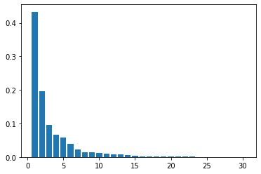
データを可視化する

pca = PCA(n_components=30)
pca.fit(X_train_scaled)
plt.bar([n for n in range(1, len(pca.explained_variance_ratio_)+1)], pca.explained_variance_ratio_)

次元数2まで圧縮

# PCA
# 次元数2まで圧縮
pca = PCA(n_components=2)
X_train_pca = pca.fit_transform(X_train_scaled)
print('X_train_pca shape: {}'.format(X_train_pca.shape))
# X_train_pca shape: (426, 2)

# 寄与率
print('explained variance ratio: {}'.format(pca.explained_variance_ratio_))
print('cumulative contribution ratio: {}'.format(pca.explained_variance_ratio_.sum()))
# explained variance ratio: [ 0.43315126  0.19586506]
# cumulative contribution ratio: 0.6290163245532956

# 散布図にプロット
temp = pd.DataFrame(X_train_pca)
temp['Outcome'] = y_train.values
b = temp[temp['Outcome'] == 0]
m = temp[temp['Outcome'] == 1]
plt.scatter(x=b[0], y=b[1], marker='o') # 良性は○でマーク
plt.scatter(x=m[0], y=m[1], marker='^') # 悪性は△でマーク
plt.xlabel('PC 1') # 第1主成分をx軸
plt.ylabel('PC 2') # 第2主成分をy軸

X_train_pca shape: (426, 2)
explained variance ratio: [0.43315126 0.19586506]
cumulative contribution ratio: 0.6290163245532956
Text(0, 0.5, 'PC 2')

形状より2次元が確認できる
また、第1成分の寄与率が0.433、第2成分の寄与率が0.195である。

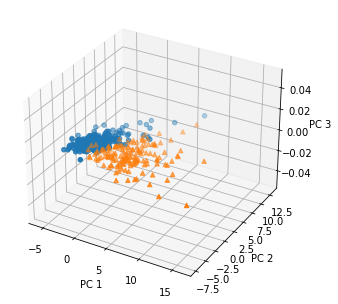
次元数3まで圧縮

pca2 = PCA(n_components=3)
X_train_pca2 = pca2.fit_transform(X_train_scaled)
print('X_train_pca2 shape: {}'.format(X_train_pca2.shape))

# 寄与率
print('explained variance ratio: {}'.format(pca2.explained_variance_ratio_))
print('cumulative contribution ratio: {}'.format(pca2.explained_variance_ratio_.sum()))

from mpl_toolkits.mplot3d import Axes3D

fig = plt.figure()
ax = Axes3D(fig)

# 散布図にプロット
temp = pd.DataFrame(X_train_pca2)
temp['Outcome'] = y_train.values
b = temp[temp['Outcome'] == 0]
m = temp[temp['Outcome'] == 1]
ax.scatter(xs=b[0], ys=b[1], marker='o') 
ax.scatter(xs=m[0], ys=m[1], marker='^') 
ax.set_xlabel('PC 1')
ax.set_ylabel('PC 2')
ax.set_zlabel('PC 3')

X_train_pca2 shape: (426, 3)
explained variance ratio: [0.43315126 0.19586506 0.09570611]
cumulative contribution ratio: 0.7247224331320569

第５章　アルゴリズム

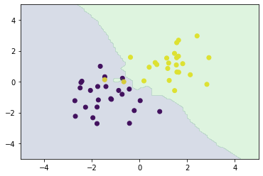
5.1 k近傍法

教師あり学習の１つ。分類問題のための機械学習手法
最近傍のデータを$k$個取り、それらが最も多く属するクラスに識別する。
$k$を変化させると結果も変わる
$k$を大きくすると決定境界は滑らかになる

第５章 k近傍法のハンズオン

課題：人口データと分類結果をプロット
モジュールのインポート

%matplotlib inline
import numpy as np
import matplotlib.pyplot as plt
from scipy import stats

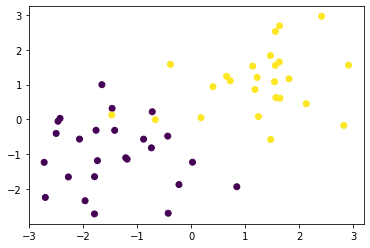
訓練データの生成

def gen_data():
    x0 = np.random.normal(size=50).reshape(-1, 2) - 1
    x1 = np.random.normal(size=50).reshape(-1, 2) + 1.
    x_train = np.concatenate([x0, x1])
    y_train = np.concatenate([np.zeros(25), np.ones(25)]).astype(np.int)
    return x_train, y_train

X_train, ys_train = gen_data()
plt.scatter(X_train[:, 0], X_train[:, 1], c=ys_train)

matplotlib.collections.PathCollection at 0x7f9ed90f2b38

# 距離の計算
def distance(x1, x2):
    return np.sum((x1 - x2)**2, axis=1)

def knc_predict(n_neighbors, x_train, y_train, X_test):
    y_pred = np.empty(len(X_test), dtype=y_train.dtype)
    for i, x in enumerate(X_test):
        distances = distance(x, X_train)
        nearest_index = distances.argsort()[:n_neighbors]
        mode, _ = stats.mode(y_train[nearest_index])
        y_pred[i] = mode
    return y_pred

# 図
def plt_resut(x_train, y_train, y_pred):
    xx0, xx1 = np.meshgrid(np.linspace(-5, 5, 100), np.linspace(-5, 5, 100))
    xx = np.array([xx0, xx1]).reshape(2, -1).T
    plt.scatter(x_train[:, 0], x_train[:, 1], c=y_train)
    plt.contourf(xx0, xx1, y_pred.reshape(100, 100).astype(dtype=np.float), alpha=0.2, levels=np.linspace(0, 1, 3))

# ハイパーパラメータk=3
n_neighbors = 3

xx0, xx1 = np.meshgrid(np.linspace(-5, 5, 100), np.linspace(-5, 5, 100))
X_test = np.array([xx0, xx1]).reshape(2, -1).T

# k近傍法
y_pred = knc_predict(n_neighbors, X_train, ys_train, X_test)
plt_resut(X_train, ys_train, y_pred)

numpyによる実装

xx0, xx1 = np.meshgrid(np.linspace(-5, 5, 100), np.linspace(-5, 5, 100))
xx = np.array([xx0, xx1]).reshape(2, -1).T

from sklearn.neighbors import KNeighborsClassifier
knc = KNeighborsClassifier(n_neighbors=n_neighbors).fit(X_train, ys_train)
plt_resut(X_train, ys_train, knc.predict(xx))

5.2 k-平均法（k-means）

$k$-平均法は教師なし学習の１つで、トップダウンでクラスタリングする機械学習の手法
$k$-平均法は教師なし学習、つまりラベルのないデータの分類方法です
与えられたデータを$k$個のクラスタリング（特徴が似ているグループ化）する。
クラスタリングのゴールは、同じクラスタ内のデータ点同士の距離が短くなるように、データを与えられた数のクラスタに分類していきます。具体的には、

$k$-平均法のアルゴリズム
１．各クラスタ中心の初期値を設定する
２．各データ点に対して、各クラスタ中心との距離を計算し、最も距離が近いクラスタを割り当てる
３．各クラスタの平均ベクトル（中心）を計算する
４．収束するまで2～3の処理を繰り返す

第５章　k-平均法のハンズオン

課題：人口データと分類結果をプロット
モジュールのインポート

%matplotlib inline
import numpy as np
import matplotlib.pyplot as plt

データ生成

def gen_data():
    x1 = np.random.normal(size=(100, 2)) + np.array([-5, -5])
    x2 = np.random.normal(size=(100, 2)) + np.array([5, -5])
    x3 = np.random.normal(size=(100, 2)) + np.array([0, 5])
    return np.vstack((x1, x2, x3))

#データ作成
X_train = gen_data()
#データ描画
plt.scatter(X_train[:, 0], X_train[:, 1])

matplotlib.collections.PathCollection at 0x7f91d7c80208

学習

def distance(x1, x2):
    return np.sum((x1 - x2)**2, axis=1)

n_clusters = 3
iter_max = 100

# 各クラスタ中心をランダムに初期化
centers = X_train[np.random.choice(len(X_train), n_clusters, replace=False)]

for _ in range(iter_max):
    prev_centers = np.copy(centers)
    D = np.zeros((len(X_train), n_clusters))
    # 各データ点に対して、各クラスタ中心との距離を計算
    for i, x in enumerate(X_train):
        D[i] = distance(x, centers)
    # 各データ点に、最も距離が近いクラスタを割り当
    cluster_index = np.argmin(D, axis=1)
    # 各クラスタの中心を計算
    for k in range(n_clusters):
        index_k = cluster_index == k
        centers[k] = np.mean(X_train[index_k], axis=0)
    # 収束判定
    if np.allclose(prev_centers, centers):
        break

クラスタリングの結果

def plt_result(X_train, centers, xx):
    #　データを可視化
    plt.scatter(X_train[:, 0], X_train[:, 1], c=y_pred, cmap='spring')
    # 中心を可視化
    plt.scatter(centers[:, 0], centers[:, 1], s=200, marker='X', lw=2, c='black', edgecolor="white")
    # 領域の可視化
    pred = np.empty(len(xx), dtype=int)
    for i, x in enumerate(xx):
        d = distance(x, centers)
        pred[i] = np.argmin(d)
    plt.contourf(xx0, xx1, pred.reshape(100, 100), alpha=0.2, cmap='spring')

y_pred = np.empty(len(X_train), dtype=int)
for i, x in enumerate(X_train):
    d = distance(x, centers)
    y_pred[i] = np.argmin(d)

xx0, xx1 = np.meshgrid(np.linspace(-10, 10, 100), np.linspace(-10, 10, 100))
xx = np.array([xx0, xx1]).reshape(2, -1).T

plt_result(X_train, centers, xx)

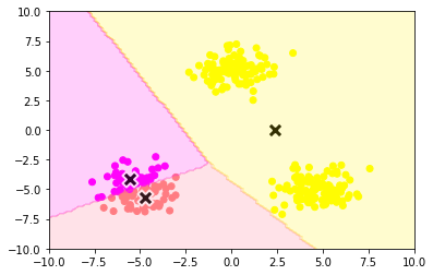
numpy実装

from sklearn.cluster import KMeans
kmeans = KMeans(n_clusters=3, random_state=0).fit(X_train)

print("labels: {}".format(kmeans.labels_))
print("cluster_centers: {}".format(kmeans.cluster_centers_))
kmeans.cluster_centers_

labels: [1 1 1 1 1 1 1 1 1 1 1 1 1 1 1 1 1 1 1 1 1 1 1 1 1 1 1 1 1 1 1 1 1 1 1 1 1
1 1 1 1 1 1 1 1 1 1 1 1 1 1 1 1 1 1 1 1 1 1 1 1 1 1 1 1 1 1 1 1 1 1 1 1 1
1 1 1 1 1 1 1 1 1 1 1 1 1 1 1 1 1 1 1 1 1 1 1 1 1 1 2 2 2 2 2 2 2 2 2 2 2
2 2 2 2 2 2 2 2 2 2 2 2 2 2 2 2 2 2 2 2 2 2 2 2 2 2 2 2 2 2 2 2 2 2 2 2 2
2 2 2 2 2 2 2 2 2 2 2 2 2 2 2 2 2 2 2 2 2 2 2 2 2 2 2 2 2 2 2 2 2 2 2 2 2
2 2 2 2 2 2 2 2 2 2 2 2 2 2 2 0 0 0 0 0 0 0 0 0 0 0 0 0 0 0 0 0 0 0 0 0 0
0 0 0 0 0 0 0 0 0 0 0 0 0 0 0 0 0 0 0 0 0 0 0 0 0 0 0 0 0 0 0 0 0 0 0 0 0
0 0 0 0 0 0 0 0 0 0 0 0 0 0 0 0 0 0 0 0 0 0 0 0 0 0 0 0 0 0 0 0 0 0 0 0 0
0 0 0 0]
cluster_centers: [[ 0.1008684 5.03166593]
[-5.11083576 -4.94058639]
[ 4.70054324 -5.00574056]]
array([[ 0.1008684 , 5.03166593],
[-5.11083576, -4.94058639],
[ 4.70054324, -5.00574056]])

plt_result(X_train, kmeans.cluster_centers_, xx)

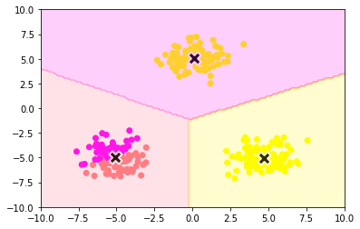
第6章　サポートベクターマシーン（SVM）

教師あり学習の１つで、2クラス分類のための機械学習手法
線形モデルの正負で2値分類

6.1 目的関数の導出

各点と決定境界との距離は、点と直線との距離の公式から

$$\frac{| w^{\rm T}x_i+b| }{ | | x | |}=\frac{t_i( w^{\rm T}x_i+b) }{ | | x | |}$$

$w$：パラメータ、$x$：説明変数、$b$：切片、$t_i$：分類

点$(\alpha ,\beta )$ と直線：$ax+by+c=0$の距離の公式は
$$\frac{|a\alpha+b\beta+c |}{\sqrt{a^2+b^2}}$$

マージンとは決定境界と最も距離の近いデータ点との距離をいい
$$\min_{i}\frac{t_i( w^{\rm T}x_i+b) }{ | | w | |}$$

サポートベクターマシーンは、マージンを最大化することを目標なので目的関数は

$$\max_{w,b}\bigg(\min_{i}\frac{t_i( w^{\rm T}x_i+b) }{ | | w | |}\bigg)$$

マージン上の点において、$t_i\left(w^{\rm T}x_i+b\right)=1$ が成り立つため、すべての点に対して、$t_i( w^{\rm T}x_i+b\geqq 1$が成り立ち、目的関数は次の式となる。
$$\max_{w.b}\frac{1}{| | w | |}$$

6.2 サポートベクターマシーンの主目的

目的関数
$$\min_{w.b}\frac12 | | w | |^2$$
制約条件
$$t_i( w^{\rm T}x_i+b\geqq 1\qquad (i=1,2,3,\cdots,n)$$

6.3 Lagrangeの未定乗数法

制約付き最適化問題を解く手法のこと。

制約条件
$$g_i(x)\geqq 0 \qquad (i=1,2,3,\cdots,n)$$
のもとで、$f(x)$ が最小となる $x$ は、変数
$\lambda_i\geqq 0\quad (i=1,2,...,n)$ を用いて新たに定義したLagrange関数
$$L(x,λ)=f(x)−\sum_{i=1}^n=\lambda_i g(x)$$
において
$$\frac{\partial L}{\partial x_j}=0\qquad (j=1,2,3,\cdots,m)$$
を満たす。

6.3.1 カルーシュ・クーン・タッカー条件

制約付き最適化問題において最適解が満たす条件のこと。

制約 $gi(x)\geqq 0\quad (i=1,2,3,\cdots,n)$ のもとで、$f(x)$ が最小となる$x^{∗}は以下を満たす。

\begin{eqnarray}
&\frac{\partial L}{\partial x_j}|_{x^*}=0\qquad (j=1,2,3,\cdots,m)\\
&g_i(x^*)\leqq 0,\quad \lambda_i \geqq 0,\quad \lambda_ig_i(x^*)\quad (i=1,2,3,\cdots,n)
\end{eqnarray}

$L$はLagrange関数、$\lambda $はLagrange乗数である

6.3.2 Lagrange関数

$$L(w,b,a)=\frac{1}{2}| | w | |^2 -\sum_{i=1}^n a_i \Big(t_i( w^{\rm T}x_i+b)-1\Big) $$
Lagrange乗数：$a_i\geqq 0\quad (i=1,2,3,\cdots,n)$

最小となる$w$、$b$ は次の式を満たす。

\begin{eqnarray}
\frac{\partial L}{\partial w}&=&w-\sum_{i=1}^na_it_ix_i=0\\
\frac{\partial L}{\partial b}&=&-\sum_{i=1} a_it_i=0
\end{eqnarray}

式変形すると

\begin{eqnarray}
w&=&\sum_{i=1}^na_it_ix_i\\
\sum_{i=1} a_it_i&=&0
\end{eqnarray}

第６章サポートベクターマシーンのハンズオン

モジュールのインポート

%matplotlib inline
import numpy as np
import matplotlib.pyplot as plt

訓練データ生成① （線形分離可能）

def gen_data():
    x0 = np.random.normal(size=50).reshape(-1, 2) - 2.
    x1 = np.random.normal(size=50).reshape(-1, 2) + 2.
    X_train = np.concatenate([x0, x1])
    ys_train = np.concatenate([np.zeros(25), np.ones(25)]).astype(np.int)
    return X_train, ys_train

X_train, ys_train = gen_data()
plt.scatter(X_train[:, 0], X_train[:, 1], c=ys_train)

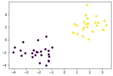
学習

t = np.where(ys_train == 1.0, 1.0, -1.0)

n_samples = len(X_train)
# 線形カーネル
K = X_train.dot(X_train.T)

eta1 = 0.01
eta2 = 0.001
n_iter = 500

H = np.outer(t, t) * K

a = np.ones(n_samples)
for _ in range(n_iter):
    grad = 1 - H.dot(a)
    a += eta1 * grad
    a -= eta2 * a.dot(t) * t
    a = np.where(a > 0, a, 0)

予測

index = a > 1e-6
support_vectors = X_train[index]
support_vector_t = t[index]
support_vector_a = a[index]

term2 = K[index][:, index].dot(support_vector_a * support_vector_t)
b = (support_vector_t - term2).mean()

xx0, xx1 = np.meshgrid(np.linspace(-5, 5, 100), np.linspace(-5, 5, 100))
xx = np.array([xx0, xx1]).reshape(2, -1).T

X_test = xx
y_project = np.ones(len(X_test)) * b
for i in range(len(X_test)):
    for a, sv_t, sv in zip(support_vector_a, support_vector_t, support_vectors):
        y_project[i] += a * sv_t * sv.dot(X_test[i])
y_pred = np.sign(y_project)

# 訓練データを可視化
plt.scatter(X_train[:, 0], X_train[:, 1], c=ys_train)
# サポートベクトルを可視化
plt.scatter(support_vectors[:, 0], support_vectors[:, 1],
                    s=100, facecolors='none', edgecolors='k')
# 領域を可視化
#plt.contourf(xx0, xx1, y_pred.reshape(100, 100), alpha=0.2, levels=np.linspace(0, 1, 3))
# マージンと決定境界を可視化
plt.contour(xx0, xx1, y_project.reshape(100, 100), colors='k',
                     levels=[-1, 0, 1], alpha=0.5, linestyles=['--', '-', '--'])


# マージンと決定境界を可視化
plt.quiver(0, 0, 0.1, 0.35, width=0.01, scale=1, color='pink')

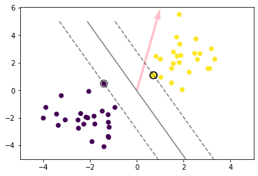
丸が付いているデータがサポートベクトル

訓練データ生成② （線形分離不可能）

factor = .2
n_samples = 50
linspace = np.linspace(0, 2 * np.pi, n_samples // 2 + 1)[:-1]
outer_circ_x = np.cos(linspace)
outer_circ_y = np.sin(linspace)
inner_circ_x = outer_circ_x * factor
inner_circ_y = outer_circ_y * factor

X = np.vstack((np.append(outer_circ_x, inner_circ_x),
               np.append(outer_circ_y, inner_circ_y))).T
y = np.hstack([np.zeros(n_samples // 2, dtype=np.intp),
               np.ones(n_samples // 2, dtype=np.intp)])
X += np.random.normal(scale=0.15, size=X.shape)
x_train = X
y_train = y

plt.scatter(x_train[:,0], x_train[:,1], c=y_train)

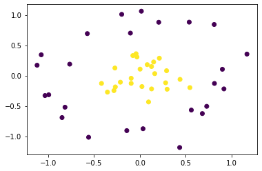
元のデータ空間では線形分離はできない（直線による分離が不可能）ため、
特徴空間上で線形分離することを考える。
今回はカーネルとしてRBFカーネル（ガウシアンカーネル）を利用する。

def rbf(u, v):
        sigma = 0.8
        return np.exp(-0.5 * ((u - v)**2).sum() / sigma**2)

X_train = x_train
t = np.where(y_train == 1.0, 1.0, -1.0)

n_samples = len(X_train)
# RBFカーネル
K = np.zeros((n_samples, n_samples))
for i in range(n_samples):
    for j in range(n_samples):
        K[i, j] = rbf(X_train[i], X_train[j])

eta1 = 0.01
eta2 = 0.001
n_iter = 5000

H = np.outer(t, t) * K

a = np.ones(n_samples)
for _ in range(n_iter):
    grad = 1 - H.dot(a)
    a += eta1 * grad
    a -= eta2 * a.dot(t) * t
    a = np.where(a > 0, a, 0)

予測

index = a > 1e-6
support_vectors = X_train[index]
support_vector_t = t[index]
support_vector_a = a[index]

term2 = K[index][:, index].dot(support_vector_a * support_vector_t)
b = (support_vector_t - term2).mean()

xx0, xx1 = np.meshgrid(np.linspace(-1.5, 1.5, 100), np.linspace(-1.5, 1.5, 100))
xx = np.array([xx0, xx1]).reshape(2, -1).T

X_test = xx
y_project = np.ones(len(X_test)) * b
for i in range(len(X_test)):
    for a, sv_t, sv in zip(support_vector_a, support_vector_t, support_vectors):
        y_project[i] += a * sv_t * rbf(X_test[i], sv)
y_pred = np.sign(y_project)

# 訓練データを可視化
plt.scatter(x_train[:, 0], x_train[:, 1], c=y_train)
# サポートベクトルを可視化
plt.scatter(support_vectors[:, 0], support_vectors[:, 1],
                    s=100, facecolors='none', edgecolors='k')
# 領域を可視化
plt.contourf(xx0, xx1, y_pred.reshape(100, 100), alpha=0.2, levels=np.linspace(0, 1, 3))
# マージンと決定境界を可視化
plt.contour(xx0, xx1, y_project.reshape(100, 100), colors='k',
                     levels=[-1, 0, 1], alpha=0.5, linestyles=['--', '-', '--'])

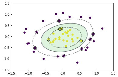
ソフトマージンSVM

訓練データ生成③（重なりあり）

x0 = np.random.normal(size=50).reshape(-1, 2) - 1.
x1 = np.random.normal(size=50).reshape(-1, 2) + 1.
x_train = np.concatenate([x0, x1])
y_train = np.concatenate([np.zeros(25), np.ones(25)]).astype(np.int)

plt.scatter(x_train[:, 0], x_train[:, 1], c=y_train)

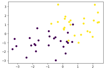
学習

X_train = x_train
t = np.where(y_train == 1.0, 1.0, -1.0)

n_samples = len(X_train)
# 線形カーネル
K = X_train.dot(X_train.T)

C = 1
eta1 = 0.01
eta2 = 0.001
n_iter = 1000

H = np.outer(t, t) * K

a = np.ones(n_samples)
for _ in range(n_iter):
    grad = 1 - H.dot(a)
    a += eta1 * grad
    a -= eta2 * a.dot(t) * t
    a = np.clip(a, 0, C)

予測

index = a > 1e-8
support_vectors = X_train[index]
support_vector_t = t[index]
support_vector_a = a[index]

term2 = K[index][:, index].dot(support_vector_a * support_vector_t)
b = (support_vector_t - term2).mean()

xx0, xx1 = np.meshgrid(np.linspace(-4, 4, 100), np.linspace(-4, 4, 100))
xx = np.array([xx0, xx1]).reshape(2, -1).T

X_test = xx
y_project = np.ones(len(X_test)) * b
for i in range(len(X_test)):
    for a, sv_t, sv in zip(support_vector_a, support_vector_t, support_vectors):
        y_project[i] += a * sv_t * sv.dot(X_test[i])
y_pred = np.sign(y_project)

# 訓練データを可視化
plt.scatter(x_train[:, 0], x_train[:, 1], c=y_train)
# サポートベクトルを可視化
plt.scatter(support_vectors[:, 0], support_vectors[:, 1],
                    s=100, facecolors='none', edgecolors='k')
# 領域を可視化
plt.contourf(xx0, xx1, y_pred.reshape(100, 100), alpha=0.2, levels=np.linspace(0, 1, 3))
# マージンと決定境界を可視化
plt.contour(xx0, xx1, y_project.reshape(100, 100), colors='k',
                     levels=[-1, 0, 1], alpha=0.5, linestyles=['--', '-', '--'])

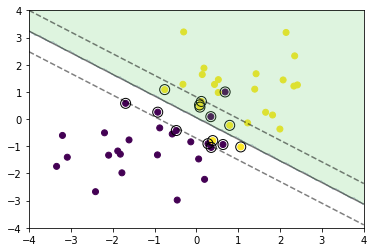
マージン内にデータが入ることを少しだけ許容して決定境界が引かれている。