概要
RBMは簡単な生成モデルとして昔からずっと興味が持ってて、今回はその推論を追いながらnumpyで実装してみた。
モデル
Energy-based Models
Energy-based Modelsとは、データセット$\mathbf{V}$の確率分布を学習するために、サンプル$\mathbf{v}$ごとにエネルギー値$E(\mathbf{v})$をつけて、確率を表示するモデルです。
p(\mathbf{v}) = \frac{e^{-E(\mathbf{v})}}{Z}
確率の高いサンプルにはエネルギー値は低い、低い確率ならはエネルギー値は高い。
よって、分配関数$Z$は
Z=\sum_\mathbf{v} e^{-E(\mathbf{v})}
Restricted Boltzmann Machines(RBM)
RBMはEnergy-based Modelsの一つである同時に、マルコフ確率場(Markov Random Field)の一つでもある。その構造はこの図のように
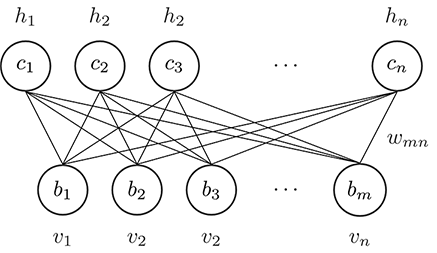
一つの**可視層(Visible Units)と隠れ層(Hidden Units)**だけの簡単な構造です。また、**Restricted(制限された)**っていうのは、接続は可視層と隠れ層の間にだけ限定されて、同じ層のUnitsはお互い独立です。
可視層と隠れ層合わせて、確率はこれになっています
p(\mathbf{v},\mathbf{h}) = \frac{e^{-E(\mathbf{v},\mathbf{h})}}{Z},
\quad
Z = \sum_\mathbf{v} \sum_\mathbf{h} e^{-E(\mathbf{v},\mathbf{h})}
エネルギー関数$E(\mathbf{v},\mathbf{h})$の定義は
\begin{aligned}
E(\mathbf{v},\mathbf{h})
&= -\mathbf{v}^\intercal W\mathbf{h} - \mathbf{b}^\intercal \mathbf{v} - \mathbf{c}^\intercal \mathbf{h} \\
&= -\sum_{i=1}^m\sum_{j=1}^n w_{ij}v_ih_j - \sum_{i=1}^m b_i v_i - \sum_{j=1}^n c_j h_j
\end{aligned}
多くの場合、隠れ層$\mathbf{h}$をベルヌーイ分布にします、すなわち$\mathbf{h} \in {0,1}^n$。
周辺分布と自由エネルギー
周辺分布$p(\mathbf{v})$を求めるなら
\begin{aligned}
p(\mathbf{v}) &= \frac{1}{Z} \sum_{\mathbf{h} \in \{0,1\}^n} \exp(\mathbf{v}^\intercal W \mathbf{h} + \mathbf{b}^\intercal \mathbf{v} + \mathbf{c}^\intercal\mathbf{h}) \\
&= \frac{1}{Z} \exp(\mathbf{b}^\intercal \mathbf{v}) \sum_{\mathbf{h}_1} \cdots \sum_{\mathbf{h}_n} \exp\left(\sum_j^n \mathbf{v}^\intercal W_{\cdot j} h_j + c_j h_j\right) \\
&= \frac{1}{Z} \exp(\mathbf{b}^\intercal \mathbf{v}) \sum_{\mathbf{h}_1} \cdots \sum_{\mathbf{h}_n} \prod_j^n \exp( \mathbf{v}^\intercal W_{\cdot j} h_j + c_j h_j) \\
&= \frac{1}{Z} \exp(\mathbf{b}^\intercal \mathbf{v}) \left(\sum_{h_1}\exp(\mathbf{v}^\intercal W_{\cdot 1} h_1 + c_1 h_1)\right) \cdots \left(\sum_{h_n}\exp(\mathbf{v}^\intercal W_{\cdot n} h_n + c_n h_n)\right) \\
&= \frac{1}{Z} \exp(\mathbf{b}^\intercal \mathbf{v}) \big(1 +\exp(\mathbf{v}^\intercal W_{\cdot 1} + c_1)\big) \cdots \big(1 +\exp(\mathbf{v}^\intercal W_{\cdot n} + c_n)\big) \\
&= \frac{1}{Z} \exp(\mathbf{b}^\intercal \mathbf{v}) \exp\Big(\log\big(1 +\exp(\mathbf{v}^\intercal W_{\cdot 1} + c_1)\big)\Big) \cdots \exp\Big(\log\big(1 +\exp(\mathbf{v}^\intercal W_{\cdot n} + c_n)\big)\Big) \\
&= \frac{1}{Z} \exp\Big(\mathbf{b}^\intercal \mathbf{v}+\sum_j^n \log\big(1 +\exp(\mathbf{v}^\intercal W_{\cdot j} + c_j)\big)\Big) \\
&= \frac{e^{-\mathcal{F}(\mathbf{v})}}{Z}
\end{aligned}
ここに出った$\mathcal{F}$は**自由エネルギー(Free Energy)**と呼びます
\mathcal{F}(\mathbf{v}) = -\mathbf{b}^\intercal \mathbf{v}-\sum_j^n \log\big(1 +\exp(\mathbf{v}^\intercal W_{\cdot j} + c_j)\big)
numpyで実装ならこうなる
def free_energy(v, W, b, c):
    first = v @ b.T
    second = (np.log(1 + np.exp(v @ W + c))).sum(axis=1,keepdims=True)
    return - first - second
条件付き分布
隠れ層$\mathbf{h}$の条件付き分布
\begin{aligned}
p(\mathbf{h}\mid \mathbf{v}) &= \frac{p(\mathbf{v},\mathbf{h})}{p(\mathbf{v})} \\
&= \frac{p(\mathbf{v},\mathbf{h})}{\sum\limits_h p(\mathbf{v},\mathbf{h})} \\
&= \frac{\frac{1}{Z}\exp(-E(\mathbf{v},\mathbf{h}))}{\sum\limits_h \frac{1}{Z}\exp(-E(\mathbf{v},\mathbf{h}))} \\
&= \frac{\exp(\mathbf{v}^\intercal W\mathbf{h} + \mathbf{b}^\intercal \mathbf{v} + \mathbf{c}^\intercal \mathbf{h})}{\sum\limits_h \exp(\mathbf{v}^\intercal W\mathbf{h} + \mathbf{b}^\intercal \mathbf{v} + \mathbf{c}^\intercal \mathbf{h})} \\
&= \frac{\exp(\mathbf{v}^\intercal W\mathbf{h})\exp(\mathbf{b}^\intercal \mathbf{v})\exp (\mathbf{c}^\intercal \mathbf{h})}{\sum\limits_h \exp(\mathbf{v}^\intercal W\mathbf{h})\exp(\mathbf{b}^\intercal \mathbf{v})\exp (\mathbf{c}^\intercal \mathbf{h})} \\
&= \frac{\exp(\mathbf{v}^\intercal W\mathbf{h})\exp (\mathbf{c}^\intercal \mathbf{h})}{\sum\limits_h \exp(\mathbf{v}^\intercal W\mathbf{h})\exp (\mathbf{c}^\intercal \mathbf{h})} \\
&= \frac{1}{Z\prime}\exp(\mathbf{v}^\intercal W\mathbf{h})\exp (\mathbf{c}^\intercal \mathbf{h}) \\
&= \frac{1}{Z\prime}\exp\big(\sum_{j=1}^n\mathbf{v}^\intercal W_{\cdot j} h_j + \sum_{j=1}^n c_j h_j\big) \\
&= \frac{1}{Z\prime} \prod_{j=1}^n \exp(\mathbf{v}^\intercal W_{\cdot j} h_j + c_j h_j) \\
&= \frac{1}{Z\prime} \prod_{j=1}^n p\prime(h_j \mid \mathbf{v})
\end{aligned}
ここまでわかるのは、同じ層のUnitsはたしかにお互い独立ですよね。そして、$p\prime(h_j \mid \mathbf{v})$はまだ正規化していないの確率分布です。
\begin{aligned}
p(h_j =1 \mid \mathbf{v}) &= \frac{p\prime(h_j=1,\mathbf{v})}{p\prime(h_j=0,\mathbf{v}) + p\prime(h_j=1,\mathbf{v})} \\
&= \frac{\exp(\mathbf{v}^\intercal W_{\cdot j} + c_j)}{\exp(0) + \exp(\mathbf{v}^\intercal W_{\cdot j} + c_j)} \\
&= sigmoid(\mathbf{v}^\intercal W_{\cdot j} + c_j)
\end{aligned}
可視層の$\mathbf{v}$も同じく
p(v_i =1 \mid \mathbf{h}) = sigmoid(W_{i \cdot} \mathbf{h} + b_j)
numpyの実装ならば
def sigmoid(x):
    return 1 / (1 + np.exp(-x))

def h_given_v(v, W, c):
    return sigmoid(v @ W + c)

def v_given_h(h, W, b):
    return sigmoid(h @ W.T + b)
損失関数
学習は最尤推定法で行います。推定したいパラメータ$\theta = {W,\mathbf{b},\mathbf{c}}$、訓練サンプル$\mathbf{v}^{(t)}$に対して、損失関数(loss function)$\mathscr{l}(\theta)$の定義は negative log likelihood です
\begin{aligned}
\mathscr{l}(\theta) &= -\log p(\mathbf{v}^{(t)}) \\
&= -\log \sum_{\mathbf{h}} p(\mathbf{v}^{(t)}, \mathbf{h}) \\
&= -\log \frac{1}{Z} \sum_{\mathbf{h}} \exp\big(-E(\mathbf{v}^{(t)},\mathbf{h})\big) \\
&= -\log \sum_{\mathbf{h}} \exp\big(-E(\mathbf{v}^{(t)},\mathbf{h})\big) + \log Z \\
&= -\log \sum_{\mathbf{h}} \exp\big(-E(\mathbf{v}^{(t)},\mathbf{h})\big) + \log \sum_{\mathbf{v},\mathbf{h}} \exp\big(-E(\mathbf{v},\mathbf{h})\big)
\end{aligned}
微分を取って
\nabla_\theta \mathscr{l}(\theta) = \underbrace{\nabla_\theta -\log \sum_{\mathbf{h}} \exp(-E(\mathbf{v}^{(t)},\mathbf{h}))}_{\text{positive phase}} + \underbrace{\nabla_\theta \log \sum_{\mathbf{v},\mathbf{h}} \exp(-E(\mathbf{v},\mathbf{h}))}_{\text{negative phase}}
Positive Phaseには
\begin{aligned}
\nabla_\theta -\log \sum_{\mathbf{h}} \exp\big(-E(\mathbf{v}^{(t)},\mathbf{h})\big) &= -\frac{1}{\sum_{\mathbf{h}} \exp(-E(\mathbf{v}^{(t)},\mathbf{h}))} \sum_h \exp(-E(\mathbf{v}^{(t)},\mathbf{h})) \frac{\partial -E(\mathbf{v}^{(t)},\mathbf{h})}{\partial \theta} \\
&= - \sum_h \frac{\exp(-E(\mathbf{v}^{(t)},\mathbf{h}))}{\sum_{\mathbf{h}} \exp(-E(\mathbf{v}^{(t)},\mathbf{h})} \frac{\partial -E(\mathbf{v}^{(t)},\mathbf{h})}{\partial \theta} \\
&= - \sum_h \frac{\frac{\exp(-E(\mathbf{v}^{(t)},\mathbf{h}))}{Z}}{\frac{\sum_{\mathbf{h}} \exp(-E(\mathbf{v}^{(t)},\mathbf{h})}{Z}} \frac{\partial -E(\mathbf{v}^{(t)},\mathbf{h})}{\partial \theta} \\
&= - \sum_h \frac{p(\mathbf{v}^{(t)},\mathbf{h})}{p(\mathbf{v}^{(t)})} \frac{\partial -E(\mathbf{v}^{(t)},\mathbf{h})}{\partial \theta} \\
&= - \sum_h p(\mathbf{h} \mid \mathbf{v}^{(t)}) \frac{\partial -E(\mathbf{v}^{(t)},\mathbf{h})}{\partial \theta} \\
&= \mathbb{E}_\mathbf{h}\left[ \frac{\partial E(\mathbf{v}^{(t)},\mathbf{h})}{\partial \theta} \middle| \mathbf{v}^{(t)} \right]
\end{aligned}
Negative Phaseには
\begin{aligned}
\nabla_\theta \log \sum_{\mathbf{v},\mathbf{h}} \exp\big(-E(\mathbf{v},\mathbf{h})\big) &= \frac{1}{\sum_{\mathbf{v},\mathbf{h}} \exp(-E(\mathbf{v},\mathbf{h}))} \sum_{\mathbf{v},\mathbf{h}}\exp(-E(\mathbf{v},\mathbf{h})) \frac{\partial -E(\mathbf{v},\mathbf{h})}{\partial \theta} \\
&= \sum_{\mathbf{v},\mathbf{h}} \frac{\exp(-E(\mathbf{v},\mathbf{h}))}{\sum_{\mathbf{v},\mathbf{h}} \exp(-E(\mathbf{v},\mathbf{h}))} \frac{\partial -E(\mathbf{v},\mathbf{h})}{\partial \theta} \\
&= \sum_{\mathbf{v},\mathbf{h}} p(\mathbf{v},\mathbf{h}) \frac{\partial -E(\mathbf{v},\mathbf{h})}{\partial \theta} \\
&= - \mathbb{E}_{\mathbf{v},\mathbf{h}}\left[\frac{\partial E(\mathbf{v},\mathbf{h})}{\partial \theta}\right]
\end{aligned}
よって、勾配は
\nabla_\theta \mathscr{l}(\theta) = \mathbb{E}_{\mathbf{h}}\left[ \frac{\partial E(\mathbf{v}^{(t)},\mathbf{h})}{\partial \theta} \middle| \mathbf{v}^{(t)} \right] - \mathbb{E}_{\mathbf{v},\mathbf{h}}\left[\frac{\partial E(\mathbf{v},\mathbf{h})}{\partial \theta}\right]
でも、第二項の$\mathbb{E}_{\mathbf{v},\mathbf{h}}$は intractable なので、近似するしかない。
Contrastive Divergence
Contrastive DivergenceはMCMCの一つである、そのコンセプトは
- $\mathbf{v}^{(t)}$を基で$k$回のギブスサンプリング (Gibbs sampling)を取って、$\tilde{\mathbf{v}}$と$\tilde{\mathbf{h}}$という negative サンプルを取得
- $\mathbb{E}_{\mathbf{v},\mathbf{h}}$を$\tilde{\mathbf{v}}$における点推定に置き換える
\mathbb{E}_{\mathbf{v},\mathbf{h}}[\nabla_\theta E(\mathbf{v},\mathbf{h})]
\approx \nabla_\theta E(\mathbf{v},\mathbf{h}) \mid_{\mathbf{v}=\tilde{\mathbf{v}},\mathbf{h}=\tilde{\mathbf{h}}}
ギブスサンプリングは二つの層に交代的に行います。
- $\mathbf{h}^{(k)} \sim p(\mathbf{h} \mid \mathbf{v}^{(k)})$
- $\mathbf{v}^{(k+1)} \sim p(\mathbf{v} \mid \mathbf{h}^{(k)})$
そして、それぞれは偏微分を取って
\nabla_W E(\mathbf{v}, \mathbf{h}) = \frac{\partial}{\partial W} - \mathbf{v}^\intercal W \mathbf{h} - \mathbf{b}^\intercal \mathbf{v} - \mathbf{c}^\intercal \mathbf{h} = - \mathbf{h} \mathbf{v}^\intercal
\nabla_\mathbf{b} E(\mathbf{v}, \mathbf{h}) = \frac{\partial}{\partial \mathbf{b}} -\mathbf{v}^\intercal W \mathbf{h} - \mathbf{b}^\intercal \mathbf{v} - \mathbf{c}^\intercal \mathbf{h} = - \mathbf{v}
\nabla_\mathbf{c} E(\mathbf{v}, \mathbf{h}) = \frac{\partial}{\partial \mathbf{c}} -\mathbf{v}^\intercal W \mathbf{h} - \mathbf{b}^\intercal \mathbf{v} - \mathbf{c}^\intercal \mathbf{h} = - \mathbf{h}
よって、各パラメーターの誤差逆伝播(Back Propagation)がわかりました。例えば、$W$の場合
\begin{aligned}
W &\Leftarrow W - \eta \big(\nabla_W - \log p(\mathbf{v}^{(t)})\big) \\
&\Leftarrow W - \eta \left(\mathbb{E}_\mathbf{h}\big[ \nabla_W E(\mathbf{v}^{(t)}, \mathbf{h}) \mid \mathbf{v}^{(t)} \big] - \mathbb{E}_{\mathbf{v},\mathbf{h}} [\nabla_W E(\mathbf{v},\mathbf{h})] \right) \\
&\Leftarrow W - \eta \left(\mathbb{E}_\mathbf{h}\big[ \nabla_W E(\mathbf{v}^{(t)}, \mathbf{h}) \mid \mathbf{v}^{(t)} \big] - \mathbb{E}_{\tilde{\mathbf{h}}} [\nabla_W E(\tilde{\mathbf{v}},\tilde{\mathbf{h}}) \mid \tilde{\mathbf{v}}] \right) \\
&\Leftarrow W - \eta \left(\mathbb{E}_\mathbf{h}\big[ -\mathbf{h}{\mathbf{v}^{(t)}}^\intercal \mid \mathbf{v}^{(t)} \big] - \mathbb{E}_\tilde{\mathbf{h}}\big[ -\tilde{\mathbf{h}}\tilde{\mathbf{v}}^\intercal \mid \tilde{\mathbf{v}} \big] \right) \\
&\Leftarrow W + \eta \left(sigmoid({\mathbf{v}^{(t)}}^\intercal W + \mathbf{c}) {\mathbf{v}^{(t)}}^\intercal - sigmoid(\tilde{\mathbf{v}}^\intercal W + \mathbf{c}) \tilde{\mathbf{v}}^\intercal \right)
\end{aligned}
バイアスの$\mathbf{b}$と$\mathbf{c}$も同じく扱うと
\mathbf{b} \Leftarrow \mathbf{b} + \eta (\mathbf{v}^{(t)} - \tilde{\mathbf{v}})
\mathbf{c} \Leftarrow \mathbf{c} + \eta \big(sigmoid({\mathbf{v}^{(t)}}^\intercal W + \mathbf{c}) - sigmoid(\tilde{\mathbf{v}}^\intercal W + \mathbf{c})\big)
さて、numpyで実装しましょう
def bernoulli(p):
    return np.floor(p + np.random.uniform(size=p.shape))

def cd_k(v, W, b, c, k=1):
    h_p = h_given_v(v, W, c)
    h = bernoulli(h_p)

    neg_v_p = v_given_h(h, W, b)
    neg_v = bernoulli(neg_v_p)
    neg_h_p = h_given_v(neg_v, W, c)
    neg_h = bernoulli(neg_h_p)

    for _ in range(k-1):
        neg_v_p = v_given_h(neg_h, W, b)
        neg_v = bernoulli(neg_v_p)
        neg_h_p = h_given_v(neg_v, W, c)
        neg_h = bernoulli(neg_h_p)

    dw = v.T @ h_p - neg_v.T @ neg_h_p
    db = v - neg_v
    dc = h - neg_h

    return dw, db, dc
Pseudo-likelihood
訓練の前にもう一つの準備が必要です。損失関数は intractable なので、代わりに Pseudo-likelihood というメトリクスを利用します。アイデアは簡単です。訓練サンプル$\mathbf{v}^{(t)}$に対して、ランダムに一つのビットを$1 \to 0$あるいは$0 \to 1$で「破壊」してnegative サンプル$\tilde{\mathbf{v}}$を得られて、そしてこの2つのサンプルの自由エネルギーの差は Pseudo-likelihood です。
\log PL(\mathbf{v}) \approx N \log\Big(sigmoid\big(\mathscr{F}(\tilde{\mathbf{v}}) - \mathscr{F}(\mathbf{v})\big)\Big)
numpy の実装
def pseudo_likelihood(v, W, b, c):
    ind = (np.arange(v.shape[0]), np.random.randint(0, v.shape[1], v.shape[0]))
    v_ = v.copy()
    v_[ind] = 1 - v_[ind]
    fe  = free_energy(v, W, b, c)
    fe_ = free_energy(v_, W, b, c)
    return (v.shape[0] * np.log(sigmoid(fe_ - fe))).mean(axis=0)
訓練
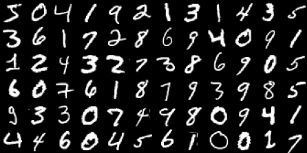
いよいよ訓練がはじめるよ、今回はmnistで試しましょう。
環境とデータ準備
import numpy as np
import seaborn as sns
import matplotlib.pyplot as plt
from sklearn.datasets import fetch_openml
from sklearn.preprocessing import minmax_scale

data, target = fetch_openml('mnist_784', version=1, return_X_y=True)

size, dim = 28, np.array([6,12])

fig, ax = plt.subplots(figsize=(6,4))

img = np.zeros(dim * size, dtype='uint8')
for i, d in enumerate(data[:dim.prod()]):
    ix, iy = divmod(i, dim[1])
    img[ix*size:(ix+1)*size, iy*size:(iy+1)*size] = d.reshape(28,28)

ax.imshow(img, cmap="gray")
ax.set_axis_off()
with plt.rc_context({"savefig.pad_inches": 0}):
    plt.show()
パラメータ設定
train_ds = data.astype(np.float32) / 255.0

def xavier_init(fan_in, fan_out, const=1.0):
    k = const * np.sqrt(6.0 / (fan_in + fan_out))
    return np.random.uniform(-k, k, (fan_in, fan_out))

batch_size = 64
n_batch = (data.shape[0] + batch_size - 1) // batch_size # ceil
n_epoch = 10
n_vis, n_hid = 784, 64
lr = 0.1
k = 1

params = {
    "W": xavier_init(n_vis, n_hid),
    "b": np.zeros([1, n_vis]),
    "c": np.zeros([1, n_hid])
}
訓練開始
for e in range(n_epoch):
    cost = []
    for v in np.array_split(train_ds, n_batch):
        dw, db, dc = cd_k(v, params['W'], params['b'], params['c'], k)
        params['W'] += (lr / v.shape[0]) * dw
        params['b'] += (lr / v.shape[0]) * db.sum(axis=0)
        params['c'] += (lr / v.shape[0]) * dc.sum(axis=0)
        cost.append(pseudo_likelihood(v, params['W'], params['b'], params['c']))

    print("Epoch: {} cost: {:.6f}".format(e, np.mean(cost)))
出力は
Epoch: 0 cost: -10.212753
Epoch: 1 cost: -8.183398
Epoch: 2 cost: -7.647802
Epoch: 3 cost: -7.483645
Epoch: 4 cost: -7.359071
Epoch: 5 cost: -7.193161
Epoch: 6 cost: -6.994519
Epoch: 7 cost: -6.987463
Epoch: 8 cost: -6.917506
Epoch: 9 cost: -7.007021
結果
学習した分布をサンプリングしましょう
def gibbs(v, W, b, c, k=1):
    h = bernoulli(h_given_v(v, W, c))
    for _ in range(k):
        v = v_given_h(h, W, b)
        h = bernoulli(h_given_v(bernoulli(v), W, c))
    return v

images = train_ds[:batch_size]
v = gibbs(images, params['W'], params['b'], params['c'], k)

size, dim = 28, np.array([8,8])

fig, ax = plt.subplots(1, 2, figsize=(8,5))

img = np.zeros(dim * size, dtype=np.float32)
for i in range(dim.prod()):
    ix, iy = divmod(i, dim[1])
    img[ix*size:(ix+1)*size, iy*size:(iy+1)*size] = images[i].reshape((28,28))
ax[0].imshow(img, cmap="gray")
ax[0].set_axis_off()
ax[0].set(title="original")

img = np.zeros(dim * size, dtype=np.float32)
for i in range(dim.prod()):
    ix, iy = divmod(i, dim[1])
    img[ix*size:(ix+1)*size, iy*size:(iy+1)*size] = v[i].reshape((28,28))
ax[1].imshow(img, cmap="gray")
ax[1].set_axis_off()
ax[1].set(title="reconstructed")

plt.tight_layout()
plt.show()
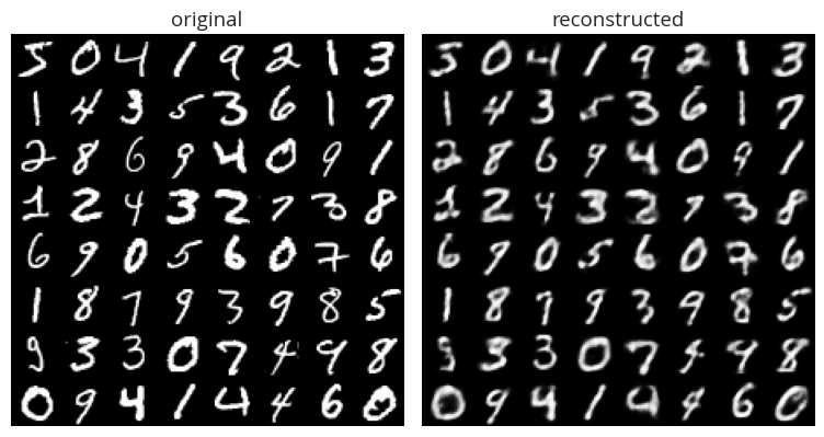
ちょっとぼけているけど、大体復元しました。
最後に、学習したモデルの中身も見てみましょう
W = minmax_scale(params['W'])
dim = np.array([8, 8])
fig, ax = plt.subplots(figsize=(6, 6))

img = np.zeros(dim * size, dtype=np.float32)
for i in range(dim.prod()):
    x, y = divmod(i, dim[1])
    img[x*size:(x+1)*size, y*size:(y+1)*size] = W[:,i].reshape(28,28)
ax.imshow(img, cmap="gray")
ax.set_axis_off()

with plt.rc_context({"savefig.pad_inches": 0}):
    plt.show()
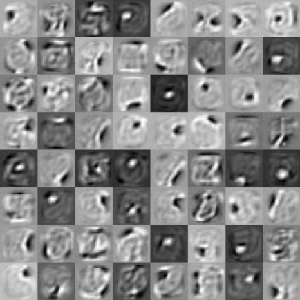
データセットを大体のそれぞれの特徴に分解したことがわかりました。
まとめ
すべての実装コードは Colab に置きました、興味ある方はそっちに参考してください。