PyTorchのチュートリアルA 60 MINUTE BLITZをやってみました
https://pytorch.org/tutorials/beginner/deep_learning_60min_blitz.html
1. インストール
公式ページに行くと環境に合わせたインストールコマンドを教えてもらえます
https://pytorch.org/get-started/locally/

上記ではPython版Stable versionをWindows + CUDA10.1環境にpipでインストールする場合のコマンドが表示されています。公式ではcondaでのインストールを推奨しているようですがpipでインストールに失敗したことがないのでpipでも大丈夫だと思います。なお、python2系は対応してないのでpython3系環境にインストールしましょう。
正常にインストールされていれば以下を実行出来る筈です
>>> import torch
>>> x = torch.rand(5, 3)
>>> print(x)

tensor([[0.4095, 0.9509, 0.5004],
        [0.7022, 0.7838, 0.8452],
        [0.6560, 0.2921, 0.4012],
        [0.1274, 0.6157, 0.4293],
        [0.2008, 0.7606, 0.0061]])
CUDAが有効になっているか確認しておきます
>>> import torch
>>> torch.cuda.is_available()
True
問題ないようです
2. tensorの扱い方
np.array的な感じで使えるようになっています
https://pytorch.org/tutorials/beginner/blitz/tensor_tutorial.html#sphx-glr-beginner-blitz-tensor-tutorial-py
2-1. torch.tensorを作る
ゼロ埋め、1埋めのtensorを作る
>>> torch.ones(2, 2)
tensor([[1., 1.],
        [1., 1.]])

>>> torch.zeros(2, 2)
tensor([[0., 0.],
        [0., 0.]])
乱数でtensorを作る
>>> torch.rand(2, 2, dtype=torch.float)
tensor([[0.0020, 0.1918],
        [0.4320, 0.5111]])
listからtensorを作る
>>> import torch
>>> import numpy as np

>>> data = [[1, 2],[3, 4]]
>>> x_data = torch.tensor(data)
>>> x_data

tensor([[1, 2],
        [3, 4]])
np.ndarrayからtensorを作る
>>> arr = np.array([[1, 2],[3, 4]])
>>> x_data = torch.tensor(arr)
>>> x_data

tensor([[1, 2],
        [3, 4]], dtype=torch.int32)
>>> x_data = torch.from_numpy(arr)
>>> x_data

tensor([[1, 2],
        [3, 4]], dtype=torch.int32)
ちなみにtorch.from_numpy()で作った場合には元のnumpy.ndarrayに何やら仕込んでくれるようで、元になったnumpy.ndarrayオブジェクトの計算結果を作ったtensorに反映することが出来ます。
>>> n = np.ones(5)
>>> t = torch.from_numpy(n)
>>> t2 = torch.tensor(n)

>>> print(f"t: {t}")
>>> print(f"n: {t2}")
>>> print(f"n: {n}", '\n')

t: tensor([1., 1., 1., 1., 1.], dtype=torch.float64)
n: tensor([1., 1., 1., 1., 1.], dtype=torch.float64)
n: [1. 1. 1. 1. 1.]

>>> np.add(n, 1, out=n)
>>> print(f"t: {t}")
>>> print(f"n: {t2}")
>>> print(f"n: {n}")

t: tensor([2., 2., 2., 2., 2.], dtype=torch.float64)
n: tensor([1., 1., 1., 1., 1.], dtype=torch.float64)
n: [2. 2. 2. 2. 2.]
tensorからnp.ndarrayを作る
numpy.arrayを作りたい場合は以下で作れます
arr = np.array(x_data)
arr
numpy()メソッドを使ってnumpy.arrayを作ることもできます
arr = x_data.numpy()
arr
こちらもnumpy()メソッドで作ったnumpy.ndarrayっぽいオブジェクトには何やら仕込まれているようで、元になったオブジェクトへの変更を反映することが出来ます。
>>> t = torch.ones(5)
>>> n = t.numpy()
>>> arr = np.array(t)

>>> print(f"t: {t}")
>>> print(f"n: {n}")
>>> print(f"arr: {arr}", '\n')

t: tensor([1., 1., 1., 1., 1.])
n: [1. 1. 1. 1. 1.]
arr: [1. 1. 1. 1. 1.]

>>> t.add_(1)
>>> print(f"t: {t}")
>>> print(f"n: {n}")
>>> print(f"arr: {arr}")

t: tensor([2., 2., 2., 2., 2.])
n: [2. 2. 2. 2. 2.]
arr: [1. 1. 1. 1. 1.]
2-2. tensorをcudaで扱えるようにする
PyTorchは同じ環境でCPUとGPUの両方が使えるようになっていて、どちらを使うのかをtensorやmodelのモード切り替えで明確にする仕組みのようです。
GPUで扱う
to('cuda')で切り替える際にCUDAデバイスへの割り当てが行われて、どのCUDAデバイスに割り当てられているかが表示されるようになります
>>> tensor = torch.tensor([[1, 2], [1, 2]])
>>> if torch.cuda.is_available():
>>>     tensor = tensor.to('cuda')
>>> tensor
tensor([[1, 2],
        [1, 2]], device='cuda:0')
to('cuda')の代わりにcuda()でも同じです
>>> tensor = tensor.cuda()
>>> tensor
tensor([[1, 2],
        [1, 2]], device='cuda:0')
CPUで扱う
CPUで扱うように戻すことも出来ます
>>> tensor = tensor.to('cpu')
>>> tensor
tensor([[1, 2],
        [1, 2]])
>>> tensor = tensor.cuda()
>>> tensor
tensor([[1, 2],
        [1, 2]])
2-3. tensorの一部を書き換える
>>> tensor = torch.ones(4, 4)
>>> tensor[:, 1] = 0
>>> tensor[3, 2] = 4
>>> print(tensor)

tensor([[1., 0., 1., 1.],
        [1., 0., 1., 1.],
        [1., 0., 1., 1.],
        [1., 0., 4., 1.]])
2-4. tensorの計算
使えるメソッドは以下にまとまっています
https://pytorch.org/docs/stable/torch.html
スカラー和
>>> arr = np.arange(6).reshape(2, 3)
>>> tensor = torch.tensor(arr)
>>> print(tensor, '\n')

tensor([[0, 1, 2],
        [3, 4, 5]], dtype=torch.int32)

>>> print(tensor + 5, '\n')
>>> print(tensor, '\n')

tensor([[ 5,  6,  7],
        [ 8,  9, 10]], dtype=torch.int32)

tensor([[0, 1, 2],
        [3, 4, 5]], dtype=torch.int32)

>>> tensor = tensor + 5
>>> print(tensor)

tensor([[ 5,  6,  7],
        [ 8,  9, 10]], dtype=torch.int32)
要素ごとの積
>>> tensor = torch.ones(4, 4)
>>> tensor[:, 1] = 0
>>> print(tensor, '\n')

tensor([[1., 0., 1., 1.],
        [1., 0., 1., 1.],
        [1., 0., 1., 1.],
        [1., 0., 1., 1.]])

>>> # This computes the element-wise product
>>> print(f"tensor.mul(tensor) \n {tensor.mul(tensor)} \n")
>>> # Alternative syntax:
>>> print(f"tensor * tensor \n {tensor * tensor}")

tensor.mul(tensor)
 tensor([[1., 0., 1., 1.],
        [1., 0., 1., 1.],
        [1., 0., 1., 1.],
        [1., 0., 1., 1.]])

tensor * tensor
 tensor([[1., 0., 1., 1.],
        [1., 0., 1., 1.],
        [1., 0., 1., 1.],
        [1., 0., 1., 1.]])
行列積
>>> print(f"tensor.matmul(tensor.T) \n {tensor.matmul(tensor.T)} \n")

tensor.matmul(tensor.T)
 tensor([[3., 3., 3., 3.],
        [3., 3., 3., 3.],
        [3., 3., 3., 3.],
        [3., 3., 3., 3.]])

>>> # Alternative syntax:
>>> print(f"tensor @ tensor.T \n {tensor @ tensor.T}")

tensor @ tensor.T
 tensor([[3., 3., 3., 3.],
        [3., 3., 3., 3.],
        [3., 3., 3., 3.],
        [3., 3., 3., 3.]])
3. autogradについて
逆誤差伝搬による微分を実現するtorch.autogradの動作を解説してくれています
https://pytorch.org/tutorials/beginner/blitz/autograd_tutorial.html#sphx-glr-beginner-blitz-autograd-tutorial-py
torch.autogradのAPIリファレンス
https://pytorch.org/docs/stable/autograd.html
3-1. 勾配の算出とoptimize
学習済みresnet18モデルに乱数で作ったデータをつっこんで勾配を算出してみましょう
モデルの読み込みとデータの作成
import numpy as np
import torch, torchvision
import matplotlib.pyplot as plt

model = torchvision.models.resnet18(pretrained=True)
data = torch.rand(1, 3, 64, 64)
labels = torch.rand(1, 1000)

arr = np.array(data)
im = np.stack([arr[0, k, :, :] for k in  range(3)], axis=2)
plt.imshow(im)
plt.show()

plt.plot(labels[0])
plt.show()
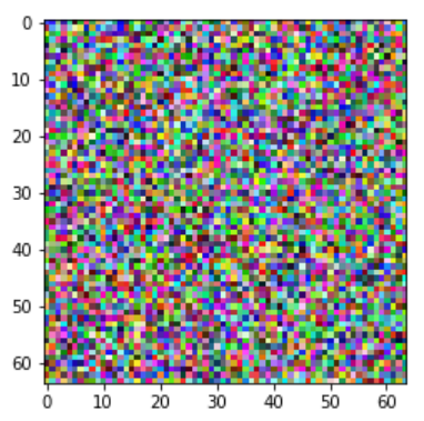
 乱数なので画像もlabelも当然意味をなさない値が入っていますがとりあえずやってみるだけなので気にしないで進めます
予測を実行
modelにデータを放り込めば推定してくれます
prediction = model(data)  # forward pass
print(prediction.shape)

plt.plot(prediction[0].detach(), label='prediction')
plt.plot(labels.numpy()[0], label='labels')
plt.legend()
plt.show()
 乱数で作った画像を放り込まれたモデルが気の毒になります
lossを算出
lossを算出します
>>> loss = (prediction - labels).sum()
>>> loss.backward() # backward pass
>>> loss

tensor(-503.5731, grad_fn=<SumBackward0>)
勾配算出の為に何やら付いてますね
optimizerを作ってパラメーターを更新する
>>> optim = torch.optim.SGD(model.parameters(), lr=1e-2, momentum=0.9)
>>> optim.step() #gradient descent
これでパラメーターの更新が完了です
実際の学習では乱数ではなく何かが写ったまともな画像と正解ラベルをバッチ枚数ごとに放り込んでいって、学習データ全体がepoch回学習されるように繰り返すわけですね。この辺、実際の画像でデモした方が分かりやすい気がするんですがこの手のライブラリを作るような人にはこれで充分ということなのかも知れません。
3-2. autogradの動作
以下のような関数を微分することを考えてみます
Q = 3a^3 + b^2
a, bで偏微分すると以下のようになります
\frac{\delta Q}{\delta a} = 9a^2 \\
\frac{\delta Q}{\delta b} = 2b
これをtorch.autogradにやってもらいましょう
a, bをつくる
import torch
a = torch.tensor([2., 3.], requires_grad=True)
b = torch.tensor([6., 4.], requires_grad=True)
a, bの関数Qをつくる
>>> Q = 3 * a ** 3 - b ** 2
>>> Q
tensor([-12.,  65.], grad_fn=<SubBackward0>)
Qの偏微分を実行
先程と同様にbackward()すれば偏微分が実行されますが、torchはloss functionのようなスカラー量が求まる関数しか偏微分できませんので、Qをどう足し合わせるか指定してやる必要があります。行列を引数として渡してやれば内積して得られた値を使ってやってくれますので、以下ではそれぞれ1倍して足し合わせた値を使ってやってくれます。
>>> external_grad = torch.tensor([1., 1.])
>>> Q.backward(gradient=external_grad)

>>> # check if collected gradients are correct
>>> print(9*a**2 == a.grad, a.grad)
>>> print(-2*b == b.grad, b.grad)

tensor([False, False]) tensor([18.0000, 40.5000])
tensor([False, False]) tensor([-6., -4.])
a, bを微分して得られる9a^2と-2bが得られているのが分かります
3-3. 微分を算出しないノードを指定する
requires_gradを省略するかrequires_grad=Falseにすると偏微分が算出されなくなります。偏微分の算出は計算コストが掛かりますので、学習する必要がないパラメーターについては偏微分を算出しないように設定するのが良いようです。
x = torch.rand(5, 5)
y = torch.rand(5, 5)
z = torch.rand((5, 5), requires_grad=True)

a = x + y
print(f"Does `a` require gradients? : {a.requires_grad}")
b = x + z
print(f"Does `b` require gradients?: {b.requires_grad}")
3-4. モデルの微分を算出しないように設定する
学習済みモデルを別のモデルに組み込んで学習をかけるような場合にモデルの学習を行わないようにするには以下のようにしてやります。model.parameters()で偉えるモデルのそれぞれのパラメーターにあたるtensorのrequires_gradをFalseにしてやるわけですね。
from torch import nn, optim

model = torchvision.models.resnet18(pretrained=True)

# Freeze all the parameters in the network
for param in model.parameters():
    param.requires_grad = False

model.fc = nn.Linear(512, 10)

# Optimize only the classifier
optimizer = optim.SGD(model.fc.parameters(), lr=1e-2, momentum=0.9)
4. CNNをやってみる
ようやく実際のneural networkのデモに到着しました
https://pytorch.org/tutorials/beginner/blitz/neural_networks_tutorial.html#sphx-glr-beginner-blitz-neural-networks-tutorial-py
4-1. ネットワークをつくる
PyTorchでは以下のような書き方でネットワークをつくるようです。クラスとして扱うのはtensorflowと同様ですが、こちらの方が書き方の自由度は高そうです。
import torch
import torch.nn as nn
import torch.nn.functional as F


class Net(nn.Module):

    def __init__(self):
        super(Net, self).__init__()
        # 1 input image channel, 6 output channels, 3x3 square convolution
        # kernel
        self.conv1 = nn.Conv2d(1, 6, 3)
        self.conv2 = nn.Conv2d(6, 16, 3)
        # an affine operation: y = Wx + b
        self.fc1 = nn.Linear(16 * 6 * 6, 120)  # 6*6 from image dimension
        self.fc2 = nn.Linear(120, 84)
        self.fc3 = nn.Linear(84, 10)

    def forward(self, x):
        # Max pooling over a (2, 2) window
        x = F.max_pool2d(F.relu(self.conv1(x)), (2, 2))
        # If the size is a square you can only specify a single number
        x = F.max_pool2d(F.relu(self.conv2(x)), 2)
        x = x.view(-1, self.num_flat_features(x))
        x = F.relu(self.fc1(x))
        x = F.relu(self.fc2(x))
        x = self.fc3(x)
        return x

    def num_flat_features(self, x):
        size = x.size()[1:]  # all dimensions except the batch dimension
        num_features = 1
        for s in size:
            num_features *= s
        return num_features


net = Net()
print(net)
畳み込み2層と全結合2層+出力1層のネットワークが構築されました
Net(
  (conv1): Conv2d(1, 6, kernel_size=(3, 3), stride=(1, 1))
  (conv2): Conv2d(6, 16, kernel_size=(3, 3), stride=(1, 1))
  (fc1): Linear(in_features=576, out_features=120, bias=True)
  (fc2): Linear(in_features=120, out_features=84, bias=True)
  (fc3): Linear(in_features=84, out_features=10, bias=True)
)
4-2. パラメーターの確認方法
parameters()メソッドでパラメーターを取得できます。weight, biasの順で入っているので5層だと10個のパラメーターがあることになります。
>>> params = list(net.parameters())
>>> print(len(params))

10
parameters()はtorch.tensor形式のパラメーターをlistに入れて出してくれるので、例えば1層目のweightは以下のようにすれば見られます
>>> print(params[0].size(), '\n')  # conv1's .weight
>>> print(params[0])

torch.Size([6, 1, 3, 3])

Parameter containing:
tensor([[[[-0.2333,  0.2431,  0.1944],
          [ 0.0508,  0.0473,  0.0961],
          [ 0.2589, -0.0621, -0.3103]]],


        [[[-0.1810, -0.3264,  0.2296],
          [ 0.1090, -0.1363,  0.2106],
          [-0.1993,  0.1884,  0.2740]]],


        [[[-0.1940,  0.2546, -0.1444],
          [ 0.2365, -0.2924,  0.0217],
          [ 0.3072, -0.0517, -0.1252]]],


        [[[ 0.3191, -0.2198, -0.1129],
          [-0.1344, -0.0281,  0.3153],
          [-0.2891,  0.1994, -0.2489]]],


        [[[ 0.2201,  0.1512, -0.2975],
          [-0.2770,  0.1493,  0.0099],
          [ 0.0210,  0.3213,  0.2986]]],


        [[[-0.0330, -0.3037, -0.0267],
          [-0.2693, -0.1042, -0.0520],
          [-0.0537, -0.2117, -0.0070]]]], requires_grad=True)
4-3. 推定する
乱数で入力データを作ってネットワークに通してみます。ネットワーク自体も初期値として入力した乱数がパラメーターとして入っているだけの意味をなさないものなので、まあなんか出てきましたというだけの出力になりますが、とりあえずのデモという事ですね。
>>> input = torch.randn(1, 1, 32, 32)
>>> out = net(input)
>>> print(out.shape, '\n')
>>> print(out)

torch.Size([1, 10])
tensor([[-0.0469,  0.0536,  0.0633, -0.0827, -0.0329,  0.0237, -0.0360,  0.0352,
         -0.0768, -0.1269]], grad_fn=<AddmmBackward>)
inputってpythonの標準関数に同じ名前のものがあるので使わない方が良い気がするんですが、まあチュートリアルなので気にせずいきましょう。
4-4. lossを算出する
以下ではloss functionとしてmseを使ってlossを算出しています
output = net(input)
target = torch.randn(10)  # a dummy target, for example
target = target.view(1, -1)  # make it the same shape as output
criterion = nn.MSELoss()

loss = criterion(output, target)
print(loss)
lossを定義するときに勾配算出の為の関数も登録されます
>>> print(loss.grad_fn)  # MSELoss
>>> print(loss.grad_fn.next_functions[0][0])  # Linear
>>> print(loss.grad_fn.next_functions[0][0].next_functions[0][0])  # ReLU

<MseLossBackward object at 0x0000020A362DF908>
<AddmmBackward object at 0x0000020A362DF708>
<AccumulateGrad object at 0x0000020A362DF908>
4-5. 勾配の算出
autogradは前回の勾配を覚えておいてbackward()したときに今回の勾配と足し合わせて返してくれますが、CNNだとその必要はないのでzero_grad()により前回の勾配を消してから微分します
>>> net.zero_grad()     # zeroes the gradient buffers of all parameters
>>> print('conv1.bias.grad before backward')
>>> print(net.conv1.bias.grad)

conv1.bias.grad before backward
tensor([0., 0., 0., 0., 0., 0.])

>>> loss.backward()
>>> print('conv1.bias.grad after backward')
>>> print(net.conv1.bias.grad)

conv1.bias.grad after backward
tensor([ 0.0004,  0.0189,  0.0209, -0.0024,  0.0032,  0.0082])
4-6. 学習の反映
例えばSGDなら以下のようにすれば更新できます
learning_rate = 0.01
for f in net.parameters():
    f.data.sub_(f.grad.data * learning_rate)
一般的なoptimizerはクラスを用意してくれていますのでそれを使えば良いようです
https://pytorch.org/docs/stable/optim.html
optimizerの定義からlossの算出、パラメーターの更新までを通してやると以下のようになります
import torch.optim as optim

# create your optimizer
optimizer = optim.SGD(net.parameters(), lr=0.01)

# in your training loop:
optimizer.zero_grad()   # zero the gradient buffers
output = net(input)
loss = criterion(output, target)
loss.backward()
optimizer.step()    # Does the update
5. まとめ
PyTorchの挙動を強く意識させる内容になっていて、tensorflowなどで既にneural networkに慣れている人向けのチュートリアルかもしれません。おかげでautogradの挙動への理解は結構進みましたが初めて触る人がここから入るとちょっと分かりにくいかも。