概要
PythonのScikit-learnで線形回帰モデルの実装手順とサンプルコードを共有する
手順
1️⃣ データの読み込み
2️⃣ 特徴量エンジニアリング
3️⃣ 説明変数 X & 目的変数 y に分割
4️⃣ train/test に分割
5️⃣ PolynomialFeatures 適用(必要に応じて)
6️⃣ StandardScaler で標準化(必要に応じて)
7️⃣ モデルの学習
8️⃣ モデルの評価
9️⃣ 可視化
🔟 モデルを保存
サンプル
サンプルコードを示す
今回は車速とアクセル開度とブレーキ開度の時系列データを与えモデルを作成した
未知の車速が与えられたときに、アクセルとブレーキ開度を予測する運転モデルを作った
sample.py
# ライブラリ
import pandas as pd
import numpy as np
from sklearn.preprocessing import PolynomialFeatures
from sklearn.preprocessing import StandardScaler
from sklearn.linear_model import LinearRegression
from sklearn.metrics import r2_score
from sklearn.model_selection import train_test_split
from sklearn.metrics import mean_squared_error
import joblib
import shap
import matplotlib.pyplot as plt
# 関数
def add_acceleration(df):
"""加速度の特徴量を追加"""
df['Acceleration[m/s2]'] = df['Speed[km/h]'].diff().fillna(0) / 3.6 / df['Time[s]'].diff().fillna(0.1)
return df
def add_feature(df, cnt):
"""数秒先の情報を特徴量に追加"""
for i in range(1, cnt): # 0.1秒, 0.2秒, 0.3秒先...
# df[f"Speed_future_{i}[km/h]"] = df['Speed[km/h]'].shift(-i)
df[f"Acceleration_future_{i}[m/s2]"] = df["Acceleration[m/s2]"].shift(-i)
return df
# 予測結果を補正
def correct_prediction(y_pred_throttle, y_pred_brake, X_test):
"""予測結果を補正"""
speed_value = X_test["Speed[km/h]"].values
# 配列をコピーして元データを変更しないようにする
y_pred_throttle_corrected = np.copy(y_pred_throttle)
y_pred_brake_corrected = np.copy(y_pred_brake)
# Speed[km/h] == 0 の場合、Throttle を 0 に補正
y_pred_throttle_corrected[speed_value == 0] = 0
# Throttle と Brake の負の値を 0 に補正
y_pred_throttle_corrected = np.maximum(y_pred_throttle_corrected, 0)
y_pred_brake_corrected = np.maximum(y_pred_brake_corrected, 0)
# `Speed[km/h] == 0` かつ `y_pred_brake < 15%` の場合、中央値(22.78%)に補正
y_pred_brake_corrected[(speed_value == 0) & (y_pred_brake_corrected < 15)] = 22.78
# アクセルとブレーキが同時に踏まれている場合、どちらか大きい方を残し、小さい方を 0 にする
mask = (y_pred_throttle_corrected > 0) & (y_pred_brake_corrected > 0)
y_pred_throttle_corrected[mask] = np.where(y_pred_throttle_corrected[mask] >= y_pred_brake_corrected[mask], y_pred_throttle_corrected[mask], 0)
y_pred_brake_corrected[mask] = np.where(y_pred_brake_corrected[mask] > y_pred_throttle_corrected[mask], y_pred_brake_corrected[mask], 0)
return y_pred_throttle_corrected, y_pred_brake_corrected
# 1️⃣ データの読み込み
df = pd.read_csv("Actual_Data.csv")
# 2️⃣ 特徴量エンジニアリング
df = add_acceleration(df)
# 未来を追加
feature_cnt = 3
df = add_feature(df, feature_cnt)
# アクセルとブレーキが同時に踏まれているデータの行数をカウント
same_time_count = ((df["Throttle[%]"] > 0) & (df["Brake[%]"] > 0)).sum()
zero_speed_throttle_count = ((df["Speed[km/h]"] == 0) & (df["Throttle[%]"] > 0)).sum()
# print(f"アクセルとブレーキが同時に踏まれている行数: {same_time_count}")
# print(f"速度0でアクセルを踏んでいる行数: {zero_speed_throttle_count}")
# データを削除
# print(f"削除前の行数: {len(df)}")
df = df[~((df["Throttle[%]"] > 0) & (df["Brake[%]"] > 0))]
df = df[~((df["Speed[km/h]"] == 0) & (df["Throttle[%]"] > 0))]
# 確認
same_time_count = ((df["Throttle[%]"] > 0) & (df["Brake[%]"] > 0)).sum()
zero_speed_throttle_count = ((df["Speed[km/h]"] == 0) & (df["Throttle[%]"] > 0)).sum()
# print(f"アクセルとブレーキが同時に踏まれている行数: {same_time_count}")
# print(f"速度0でアクセルを踏んでいる行数: {zero_speed_throttle_count}")
# NaNを削除
num_nan_rows = df.isna().any(axis=1).sum()
# print(f"NaN を含む行の数: {num_nan_rows}")
df = df.dropna()
# 確認
num_nan_rows = df.isna().any(axis=1).sum()
# print(f"NaN を含む行の数: {num_nan_rows}")
# print(f"削除後の行数: {len(df)}")
# 3️⃣ 説明変数 X & 目的変数 y に分割
xcol = ['Speed[km/h]', 'Acceleration[m/s2]', 'Acceleration_future_2[m/s2]']
X = df[xcol]
y = y = df[['Throttle[%]', 'Brake[%]']]
# 4️⃣ train/test に分割(trainが学習用、testが評価用、xが説明変数、yが目的変数)
X_train, X_test, y_train, y_test = train_test_split(X, y, test_size=0.2, random_state=42)
# 5️⃣ PolynomialFeatures 適用(必要に応じて)
poly = PolynomialFeatures(degree=3, include_bias=False)
# PolynomialFeatures を適用(train のみ fit)
X_train_poly = poly.fit_transform(X_train)
X_test_poly = poly.transform(X_test)
# 6️⃣ StandardScaler で標準化(必要に応じて)
scaler = StandardScaler()
# StandardScaler を適用(train のみ fit)
X_train_scaled = scaler.fit_transform(X_train_poly)
X_test_scaled = scaler.transform(X_test_poly)
# 7️⃣ モデルの学習
model_throttle = LinearRegression() # 切片なしならfit_intercept=False
model_brake = LinearRegression()
model_throttle.fit(X_train_scaled, y_train["Throttle[%]"])
model_brake.fit(X_train_scaled, y_train["Brake[%]"])
# 8️⃣ モデルの評価
y_pred_throttle = model_throttle.predict(X_test_scaled)
y_pred_brake = model_brake.predict(X_test_scaled)
# 補正
y_pred_throttle_corrected, y_pred_brake_corrected = correct_prediction(y_pred_throttle, y_pred_brake, X_test)
# 評価(R^2)
throttle_score = r2_score(y_test["Throttle[%]"], y_pred_throttle_corrected)
brake_score = r2_score(y_test["Brake[%]"], y_pred_brake_corrected)
# 評価(RMSE)
rmse_throttle = np.sqrt(mean_squared_error(y_test["Throttle[%]"], y_pred_throttle_corrected))
rmse_brake = np.sqrt(mean_squared_error(y_test["Brake[%]"], y_pred_brake_corrected))
print(f"Throttle R^2 Score: {throttle_score}")
print(f"Brake R^2 Score: {brake_score}")
print(f"Throttle RMSE: {rmse_throttle}")
print(f"Brake RMSE: {rmse_brake}")
# 9️⃣ 可視化
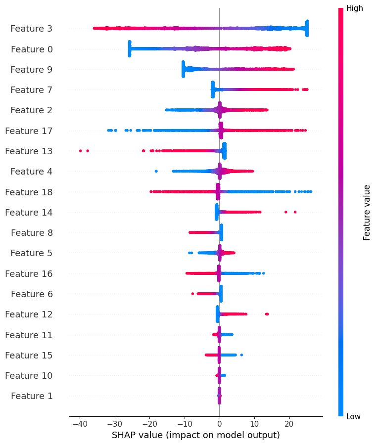
# 特徴量の重要度を SHAP などで可視化
explainer = shap.Explainer(model_throttle, X_test_scaled)
shap_values = explainer(X_test_scaled)
shap.summary_plot(shap_values, X_test_scaled)
# 回帰式の係数と切片をdfに格納
df_coef = pd.DataFrame()
feature_names = poly.get_feature_names_out(list(X.columns))
df_coef["Feature"] = feature_names
df_coef["Throttle"] = model_throttle.coef_
df_coef["Brake"] = model_brake.coef_
# csvに出力
df_coef.to_csv("coef.csv", index=False)
print("回帰式")
print(f"切片:Throttle {model_throttle.intercept_}")
print(f"切片:Brake {model_brake.intercept_}")
df_coef
# 回帰式の係数の分析
# 大きい順にソート
df_coef_throttle = df_coef.sort_values(by="Throttle", ascending=False)
df_coef_brake = df_coef.sort_values(by="Brake", ascending=False)
# グラフ表示
# グラフのサイズを設定
plt.figure(figsize=(8, 5))
# 横棒グラフを作成
plt.barh(df_coef_throttle["Feature"], df_coef_throttle["Throttle"], color="blue", edgecolor="black")
plt.title("Throttle")
# グリッドを表示(X軸方向のみ)
plt.grid(axis="x", linestyle="--", alpha=0.7)
plt.show()
# 横棒グラフを作成
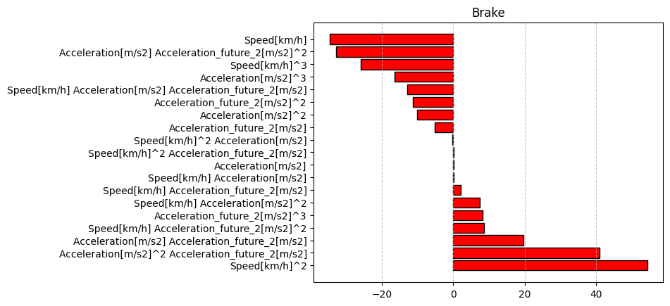
plt.barh(df_coef_brake["Feature"], df_coef_brake["Brake"], color="red", edgecolor="black")
plt.title("Brake")
# グリッドを表示(X軸方向のみ)
plt.grid(axis="x", linestyle="--", alpha=0.7)
plt.show()
# 🔟 モデルを保存
# モデルを保存(Throttle と Brake)
joblib.dump(model_throttle, "model_throttle.pkl")
joblib.dump(model_brake, "model_brake.pkl")
print("モデルが保存されました")
# モデルを読み込む
model_throttle_loaded = joblib.load("model_throttle.pkl")
model_brake_loaded = joblib.load("model_brake.pkl")
print("モデルが読み込まれました")
結果
Throttle R^2 Score: 0.9906606414122686
Brake R^2 Score: 0.9508386434187767
Throttle RMSE: 0.7252065372965398
Brake RMSE: 1.8993579634510172
回帰式
切片:Throttle 10.95503148550699
切片:Brake    4.419940406452666