はじめに
このブログはAidemy Premiumのカリキュラムの一環であり、受講修了条件を満たすために公開しています。
まず、簡単に自己紹介させていただきます。私はファームウェアやアプリケーション開発に20年以上携わっており、田舎暮らしを始めるために転職を決意しました。AI開発スキルを身につけ、これまでのソフトウェア開発経験を活かし、新たな分野で活躍することを目指しています。
目次
概要
Aidemy PremiumでCNN(Convolutional Neural Network)を用いたモデルの構築や運用、そしてVGG16を用いた転移学習について学びました。田舎での生活では150坪の農地を所有し、家庭菜園をする予定です。そのようなこともあり、農業に関連する画像識別をテーマにしたデータセットを探しました。その結果、KaggleのTomato Leaves Datasetを使用し、トマトの葉の病気を予測できる軽量モデルを開発しました。また、このモデルをFlaskで統合し、Renderに展開するWebアプリを作成することを目標としています。
実行環境
Google Colaboratory
データの収集
データセットのダウンロード
事前に、KaggleのTomato Leaves Datasetのサイト右上のDownloadボタンから、データセットのzipファイルをGoogle Driveにダウンロードしておきます。
下記のコードによって、ダウンロードしたデータセットをGoogle Colaboratoryのカレントディレクトリに展開します。
from google.colab import drive
import zipfile

# Google Driveをマウント
drive.mount('/content/drive')

# ダウンロードしたzipファイルを展開
zfile = zipfile.ZipFile('/content/drive/MyDrive/Colab Notebooks/datasets/tomato_leaves_dataset.zip')
zfile.extractall('./dataset')
展開したフォルダの内容を確認します。
datasetフォルダの中には、trainフォルダとvalidフォルダがあり、さらに各フォルダには11個のサブフォルダがあります。各サブフォルダの中には、PNG、JPG形式の画像ファイルが格納されています。
dataset
├── train
│   ├── Bacterial_spot
│   ├── Early_blight
│   ├── Late_blight
│   ├── Leaf_Mold
│   ├── Septoria_leaf_spot
│   ├── Spider_mites Two-spotted_spider_mites
│   ├── Target_Spot
│   ├── Tomoto_Yellow_Leaf_Curl_virus
│   ├── Tomoto_mosaic_virus
│   ├── healthy
│   ├── powdery_mildew
├── valid
│   ├── Bacterial_spot
│   ├── Early_blight
│   ├── Late_blight
│   ├── Leaf_Mold
│   ├── Septoria_leaf_spot
│   ├── Spider_mites Two-spotted_spider_mites
│   ├── Target_Spot
│   ├── Tomoto_Yellow_Leaf_Curl_virus
│   ├── Tomoto_mosaic_virus
│   ├── healthy
│   ├── powdery_mildew
分類するクラス
これら11個のサブフォルダ名が、分類するクラス名となります。
各クラス名の日本語訳は、上から順に以下のようになっています。
- 細菌性斑点(Bacterial_spot)
- 早期病害(Early_blight)
- 晩枯病(Late_blight)
- 葉カビ(Leaf_Mold)
- セプトリア葉斑病(Septoria_leaf_spot)
- ハダニ類 二斑点性ハダニ(Spider_mites Two-spotted_spider_mites)
- ターゲットスポット(Target_Spot)
- トマト黄化葉巻病(Tomoto_Yellow_Leaf_Curl_virus)
- トマトモザイクウイルス(Tomoto_mosaic_virus)
- 健康(healthy)
- うどんこ病(powdery_mildew)
trainフォルダのデータのうち80%を訓練データ、20%を検証データに使用します。
validフォルダのデータはテストデータとして使用します。
念のため、以下のコードでtrainフォルダとvalidフォルダのサブフォルダに差分がないことを確認しました。
import os

# 訓練データのディレクトリパス
import os

train_data_path = '/content/dataset/train'
test_data_path = '/content/dataset/valid'

assert os.listdir(train_data_path) == os.listdir(test_data_path), '分類クラス不一致'

# クラス名のリストを昇順で取得
class_names = sorted(os.listdir(train_data_path))
print('\n'.join(class_names))
実行結果として取得したクラス名のリストを変数class_namesに代入しておきます。
[実行結果]
Bacterial_spot
Early_blight
Late_blight
Leaf_Mold
Septoria_leaf_spot
Spider_mites Two-spotted_spider_mite
Target_Spot
Tomato_Yellow_Leaf_Curl_Virus
Tomato_mosaic_virus
healthy
powdery_mildew
データの前処理
データのロード
各画像の画像データと、各画像が分類されるクラスを数値化したラベルを取得するために、Image Classifierクラスを実装しました。
Image Classifierクラス
このクラスは、クラス名のリストと画像サイズで初期化されます。load_dataメソッドでは、trainフォルダやvalidフォルダのディレクトリパスから画像データをロードし、各画像のクラスに対応する数値化ラベルを返します。

各メソッドの説明は以下の通りです。
| メソッド名 | 説明 |
|---|---|
| __init__() | クラス名のリストと画像サイズを指定して、ImageClassifierクラスのインスタンスを初期化します。 |
| load_data() | データパスから画像データをロードし、それぞれの画像に対応するラベルを含むタプルを返します。 |
| get_image_paths() | データパスから画像ファイルのパスをリストで取得します。 |
| __read_image() | 画像データを読み込んで、numpy.ndarray形式で返します。 |
| __get_label() | 画像に対応するラベルを取得し、その数値を返します。 |
コードを表示する
import numpy as np
import os
import cv2

class ImageClassifier:
    '''
    データセットのデータロードと前処理を行うクラス
    '''
    def __init__(self, class_names: list, image_size: tuple=(128, 128, 3)):
        '''
        ImageClassifierクラスを初期化する

        Parameters
        ----------
        class_names : list
            クラス名のリスト
        image_size : tuple
            画像サイズ(高さ、幅、チャネル)
        '''
        self.class_names = class_names
        self.image_size = image_size

    def load_data(self, data_path):
        '''
        画像データを読み込み、データとラベル付けされた値を返す
        '''
        image_paths = self.get_image_paths(data_path)

        print('loading images and labels')

        # 画像データ、ラベルの数を格納するリスト
        images = np.empty((len(image_paths),) + self.image_size, dtype=np.uint8)
        labels = np.empty((len(image_paths),), dtype=np.uint8)

        for i, image_path in enumerate(image_paths):
            images[i] = self.__read_image(image_path)
            labels[i] = self.__get_label(image_path)

        print('loaded images', images.shape, 'labels', labels.shape)
        return images, labels

    def get_image_paths(self, data_path):
        '''
        画像ファイルのパスをリストで取得する
        '''
        paths = []
        for i in self.class_names:
            class_path = os.path.join(data_path, i)
            for j in os.listdir(class_path):
                path = os.path.join(class_path, j)
                paths.append(path)
        return paths

    def __read_image(self, image_path):
        '''
        画像データを読み込む
        '''
        image = cv2.imread(image_path)
        image = cv2.resize(image, self.image_size[:2])
        return image

    def __get_label(self, image_path):
        '''
        ラベルとしてクラス名に割り当てられた値を取得する
        '''
        # ファイル名を除いたパスの末尾からクラス名を取得
        class_name = os.path.split(image_path)[0].split('/')[-1]

        # リストの並び順をラベル付けした値として返す
        return self.class_names.index(class_name)
データの可視化
画像による可視化
Image Classifierを使って、データセットにどのような画像が含まれているかを確認すると、以下のようになりました。

グラフによる可視化
Image Classifierを使って、各クラスの画像数を棒グラフで可視化すると、以下のようになります。

このグラフを表示するために実装したコードは以下の通りです。
from collections import Counter
import matplotlib.pyplot as plt

# 画像ファイルパスを取得するためにImageClassifierのインスタンスを生成
img_classifier = ImageClassifier(class_names)

plt.title('Number of images')

for i, j in enumerate([train_data_path, test_data_path]):
    # trainフォルダもしくはvalidフォルダのパスからクラス名のリストを取得する
    paths = img_classifier.get_image_paths(j)
    class_name_list = [os.path.split(x)[0].split('/')[-1] for x in paths]

    # クラス名の出現回数をカウントして、降順に並び替える
    counts = Counter(class_name_list)
    sorted_counts = counts.most_common()

    # 要素と出現回数をそれぞれ別のリストに格納する
    elements = [item[0] for item in sorted_counts]
    frequencies = [item[1] for item in sorted_counts]

    # 棒グラフを作成する
    plt.bar(elements, frequencies, align='edge', width=0.4-0.8*i)

plt.legend(['train', 'test'])
plt.xticks(rotation=90)
plt.show()
モデルの実装
モデルのトレーニングをプログラムする際に、Kerasのモデルクラスのインスタンスをメンバーとして持つModel Wrapperクラスを定義しました。このクラスは、学習済みモデルのファイルパスと画像サイズで初期化されます。
クラス図は以下の通りです。

各メソッドの説明は以下の通りです。
| メソッド名 | 説明 |
|---|---|
| __init__() | モデルのパスと入力形状を指定して、ModelWrapperクラスのインスタンスを初期化します。 |
| train() | トレーニングデータを使用してモデルをトレーニングし、損失と精度の履歴を記憶します。 |
| save() | 学習済みモデルを保存します。 |
| evaluate() | テストデータを使用してモデルを評価し、損失と精度を可視化します。 |
| predict() | 画像データを使用してモデルによる予測を実行し、混同行列を可視化します。 |
CNN
まず初めに、Model Wrapperクラスに、以下のような構造のモデルを構築して、モデルをトレーニングしました。
Model: "sequential"
_________________________________________________________________
 Layer (type)                Output Shape              Param #
=================================================================
 rescaling (Rescaling)       (None, 128, 128, 3)       0

 conv2d (Conv2D)             (None, 128, 128, 32)      896

 max_pooling2d (MaxPooling2  (None, 64, 64, 32)        0
 D)

 conv2d_1 (Conv2D)           (None, 64, 64, 64)        18496

 max_pooling2d_1 (MaxPoolin  (None, 32, 32, 64)        0
 g2D)

 conv2d_2 (Conv2D)           (None, 32, 32, 128)       73856

 max_pooling2d_2 (MaxPoolin  (None, 16, 16, 128)       0
 g2D)

 conv2d_3 (Conv2D)           (None, 16, 16, 256)       295168

 max_pooling2d_3 (MaxPoolin  (None, 8, 8, 256)         0
 g2D)

 conv2d_4 (Conv2D)           (None, 8, 8, 512)         1180160

 max_pooling2d_4 (MaxPoolin  (None, 4, 4, 512)         0
 g2D)

 dropout (Dropout)           (None, 4, 4, 512)         0

 flatten (Flatten)           (None, 8192)              0

 dense (Dense)               (None, 512)               4194816

 dropout_1 (Dropout)         (None, 512)               0

 dense_1 (Dense)             (None, 256)               131328

 dropout_2 (Dropout)         (None, 256)               0

 dense_2 (Dense)             (None, 128)               32896

 dropout_3 (Dropout)         (None, 128)               0

 dense_3 (Dense)             (None, 64)                8256

 dropout_4 (Dropout)         (None, 64)                0

 dense_4 (Dense)             (None, 32)                2080

 dropout_5 (Dropout)         (None, 32)                0

 dense_5 (Dense)             (None, 11)                363

=================================================================
Total params: 5938315 (22.65 MB)
Trainable params: 5938315 (22.65 MB)
Non-trainable params: 0 (0.00 Byte)
_________________________________________________________________
モデルの学習
モデルの学習のために実装したコードは以下の通りです。
# Image Classifierのインスタンス化
img_classifier = ImageClassifier(class_names, (128, 128, 3))

# 画像データをロードする
images, labels = img_classifier.load_data(train_data_path)

X_train, X_test, y_train, y_test = train_test_split(
    images, labels, test_size=0.2, random_state=23, shuffle=True)

y_train = tf.keras.utils.to_categorical(y_train)
y_test = tf.keras.utils.to_categorical(y_test)

# モデルのインスタンス化
model_wrapper = ModelWrapper()

# モデルのトレーニングとトレーニング結果の保存
model_wrapper.train(X_train, y_train, (X_test, y_test), epochs=30)
モデルの評価
validフォルダのテスト用画像データを使用して、ModelWrapper.evaluateメソッドでモデルを評価しました。その結果、画像の識別精度は約90%でした。

モデルによる予測
validフォルダのテスト用画像データを使用して、混同行列を可視化した結果は以下の通りです。
とてもいい感じで画像識別できていると思いましたが、チューターの方からAIが背景画像に焦点を当てて画像識別している可能性があると指摘されました。

それを調べるためには、Grad-CAM(Gradient-weighted Class Activation Mapping)と呼ばれる手法を使用しました。Grad-CAMは、畳み込みニューラルネットワークモデルの特徴マップに基づいて、モデルがどの部分に注目して予測を行っているかを可視化します。
Grad-CAMを使用してAIの注目点を可視化するためのコードは以下の通りです。
import numpy as np
import matplotlib.pyplot as plt
import tensorflow as tf
import cv2

def make_gradcam_heatmap(image, model, last_conv_layer_name):
    '''
    Grad-CAMによるヒートマップを作成する

    Parameters
    ----------
    image : array
            画像データ
    model : class
            kerasのモデルインスタンス
    last_conv_layer_name : str
            出力に最も近い畳み込み層の名前

    Returns
    ---------
    array
            ヒートマップ画像データ
    '''
    last_conv_layer = model.get_layer(last_conv_layer_name)
    grad_model = tf.keras.models.Model([model.inputs], [last_conv_layer.output, model.output])

    with tf.GradientTape() as tape:
        last_conv_layer_output, model_output = grad_model(image)
        print('last_conv_layer_output.shape', last_conv_layer_output.shape,
              'model_output.shape', model_output.shape)
        pred_index = np.argmax(model_output[0])
        print('pred_index:', pred_index)
        class_channel = model_output[:, pred_index]
        print('class_channel', class_channel.numpy())

    grads = tape.gradient(class_channel, last_conv_layer_output)
    pooled_grads = tf.reduce_mean(grads, axis=(0, 1, 2))

    heatmap = last_conv_layer_output[0] @ pooled_grads[..., tf.newaxis]
    heatmap = tf.squeeze(heatmap)
    heatmap = tf.maximum(heatmap, 0) / tf.math.reduce_max(heatmap)
    return heatmap

def compose_heatmap(img, heatmap):
    '''
    元画像とヒートマップ画像を合成する
    '''
    INTENSITY = 0.6

    heatmap = cv2.resize(heatmap, (img.shape[1], img.shape[0]))
    heatmap = cv2.applyColorMap(np.uint8(255*heatmap), cv2.COLORMAP_JET)

    img = heatmap * INTENSITY + img

    cv2.imwrite('heatmap.jpg', img)

# テストデータをロードする
images, labels = img_classifier.load_data(test_data_path)

# ランダムに画像データを取得
index = np.random.randint(0, images.shape[0])
image = images[index]
label = labels[index]

plt.figure(figsize=(12, 4))

# 加工前の画像を表示
plt.subplot(1, 3, 1)
plt.imshow(image)
plt.title('{} ({})'.format(class_names[label], label))
plt.axis('off')

# ヒートマップ画像を作成
target_image = image.reshape(-1, 128, 128, 3)
model = tf.keras.models.load_model('/content/drive/MyDrive/Colab Notebooks/my_model.keras')
heatmap = make_gradcam_heatmap(target_image, model, 'conv2d_9')

# ヒートマップを表示
plt.subplot(1, 3, 2)
# matshowではグラフの複数表示ができなかったのでimshowを使う
#plt.matshow(heatmap)
plt.imshow(heatmap, cmap='viridis')
plt.axis('off')

compose_heatmap(image, np.array(heatmap))

# ヒートマップ合成画像を表示
plt.subplot(1, 3, 3)
img = cv2.imread('heatmap.jpg')
img = cv2.cvtColor(img, cv2.COLOR_BGR2RGB)
plt.imshow(img)
plt.axis('off')
plt.show()
上記のコードを実行したところ、いくつかの画像で背景画像に焦点を当てて画像認識していることが分かりました。


対策として、データの前処理で背景画像を除去することを検討しましたが、画像データをロードしながら背景画像を除去するのに、データ数が多い場合に膨大な時間を要したため、現実的ではないと判断しました。
以下の表に、モデルが前景画像である葉の病気の状態に着目するための施策をまとめました。
この中から、転移学習、データ拡張、カスタムレイヤーである中央クロップレイヤーをModelWrapperクラスに実装しました。
| 施策 | 期待する結果 | 実施可否 |
|---|---|---|
| 背景画像の除去 | データの前処理において、背景画像を除去することで、モデルが前傾画像である葉に焦点を当てるようにする。 | 否 |
| 転移学習 | 事前に学習されたCNNモデルを使用して葉の病気の特徴を学習。例えば、ImageNetなどのデータセットで事前学習されたモデルを使用し、転移学習を行う。 | 可 |
| データ拡張 | 病気の葉のさまざまな状態を模倣するため、データ拡張を導入。画像の回転、拡大縮小、明るさの変更などの操作を行い、より多くの病気の葉の状態を学習する。 | 可 |
| 中央クロップレイヤー | 入力画像の中央部を切り取ることで、モデルがより重要な情報に焦点を当てるようにする。 | 可 |
| 誤認識画像の削除 | 手作業で背景画像に焦点を当てた画像を削除することで、モデルの誤認識を減らす。 | 否 |
転移学習
上記の施策から、転移学習、データ拡張、中央クロップレイヤーを組み合わせて、Model Wrapperクラスに以下のようなモデルを構築しました。
_________________________________________________________________
 Layer (type)                Output Shape              Param #
=================================================================
 input_1 (InputLayer)        [(None, 128, 128, 3)]     0

 central_crop_layer (Centra  (None, 64, 64, 3)         0
 lCropLayer)

 rescaling (Rescaling)       (None, 64, 64, 3)         0

 block1_conv1 (Conv2D)       (None, 64, 64, 64)        1792

 block1_conv2 (Conv2D)       (None, 64, 64, 64)        36928

 block1_pool (MaxPooling2D)  (None, 32, 32, 64)        0

 block2_conv1 (Conv2D)       (None, 32, 32, 128)       73856

 block2_conv2 (Conv2D)       (None, 32, 32, 128)       147584

 block2_pool (MaxPooling2D)  (None, 16, 16, 128)       0

 block3_conv1 (Conv2D)       (None, 16, 16, 256)       295168

 block3_conv2 (Conv2D)       (None, 16, 16, 256)       590080

 block3_conv3 (Conv2D)       (None, 16, 16, 256)       590080

 block3_pool (MaxPooling2D)  (None, 8, 8, 256)         0

 block4_conv1 (Conv2D)       (None, 8, 8, 512)         1180160

 block4_conv2 (Conv2D)       (None, 8, 8, 512)         2359808

 block4_conv3 (Conv2D)       (None, 8, 8, 512)         2359808

 block4_pool (MaxPooling2D)  (None, 4, 4, 512)         0

 block5_conv1 (Conv2D)       (None, 4, 4, 512)         2359808

 block5_conv2 (Conv2D)       (None, 4, 4, 512)         2359808

 block5_conv3 (Conv2D)       (None, 4, 4, 512)         2359808

 block5_pool (MaxPooling2D)  (None, 2, 2, 512)         0

 sequential (Sequential)     (None, 11)                2109451

=================================================================
Total params: 16824139 (64.18 MB)
Trainable params: 2109451 (8.05 MB)
Non-trainable params: 14714688 (56.13 MB)
_________________________________________________________________
コードを表示する
import numpy as np
import matplotlib.pyplot as plt
import pickle
import tensorflow as tf
from sklearn.metrics import confusion_matrix
from sklearn.metrics import accuracy_score, precision_score, recall_score, f1_score
from google.colab import files

# 中央クロップレイヤーの定義
@tf.keras.utils.register_keras_serializable()
class CentralCropLayer(tf.keras.layers.Layer):
    def __init__(self, crop_size):
        super(CentralCropLayer, self).__init__()
        self.crop_size = crop_size

    def call(self, inputs):
        cropped_images = tf.image.central_crop(inputs, central_fraction=self.crop_size)
        return cropped_images

class ModelWrapper:
    '''
    CNNによって画像認識の学習・評価・予測を行うモデルのWrapperクラス
    '''
    def __init__(self, model_path=None, input_shape=(128, 128, 3)):
        '''
        ModelWrapper クラスを初期化する
        '''
        self.model = None
        self.history = {}

        try:
            if model_path is not None:
                self.model = tf.keras.models.load_model(model_path)
            else:
                input_tensor = tf.keras.Input(shape=input_shape)

                # 中央クロップレイヤー
                central_crop_layer = CentralCropLayer(0.5)
                cropped_input = central_crop_layer(input_tensor)

                # Rescalingレイヤー
                rescaling_layer = tf.keras.layers.Rescaling(scale=1./255)(cropped_input)

                # VGG16モデルをロード
                vgg16_model = tf.keras.applications.VGG16(
                    weights='imagenet',
                    include_top=False,
                    input_tensor=rescaling_layer)

                # VGG16モデルの最後の層の直前までの出力を凍結する
                for layer in vgg16_model.layers:
                    layer.trainable = False

                # 全結合層を追加する
                top_model = tf.keras.Sequential([
                    tf.keras.layers.Flatten(input_shape=vgg16_model.output_shape[1:]),
                    tf.keras.layers.Dense(1024, activation='relu'),
                    tf.keras.layers.Dropout(0.5),
                    tf.keras.layers.Dense(len(class_names), activation='softmax')
                ])

                # 新しいモデルを定義
                self.model = tf.keras.Model(
                    inputs=input_tensor,
                    outputs=top_model(vgg16_model.output))
        except Exception as e:
            print(f'モデルの読み込み中にエラーが発生しました: {e}')
        else:
            self.model.summary()

    def train(self, X_train, y_train, validation_data,
              epochs=30, batch_size=128, verbose=1):
        '''
        モデルをトレーニングする
        '''
        initial_learning_rate = 0.001
        steps_per_epoch = int(len(X_train) / batch_size)
        print('steps_per_epoch:', steps_per_epoch)
        # 学習率スケジューラーの定義
        learning_rate_scheduler = tf.keras.optimizers.schedules.ExponentialDecay(
            initial_learning_rate=initial_learning_rate,
            decay_steps=steps_per_epoch * 10,
            decay_rate=0.96
        )

        # 最適化アルゴリズムと学習率スケジューラーを組み合わせて使用
        optimizer = tf.keras.optimizers.Adam(learning_rate=learning_rate_scheduler)
        self.model.compile(
            optimizer=optimizer,
            loss='categorical_crossentropy',
            metrics=['accuracy']
        )

        # データ拡張の設定
        datagen = tf.keras.preprocessing.image.ImageDataGenerator(
            rotation_range=15,
            width_shift_range=0.1,
            height_shift_range=0.1,
            horizontal_flip=True
        )
        datagen.fit(X_train)

        # 早期終了の設定
        early_stopping = tf.keras.callbacks.EarlyStopping(monitor='val_loss', patience=5)

        print('train started')
        history = self.model.fit(
            datagen.flow(X_train, y_train, batch_size=batch_size),
            steps_per_epoch=len(X_train) // batch_size,
            epochs=epochs,
            validation_data=validation_data,
            verbose=verbose,
            callbacks=[early_stopping]
        )
        print('train finished')

        self.history = history.history

    def save(self, model_filename=None):
        '''
        学習済みモデルを保存する
        '''
        if model_filename is not None:
            self.model.save(model_filename)
            files.download(os.path.join(os.getcwd(), model_filename))

    def evaluate(self, X_test, y_test, batch_size=128, verbose=1):
        '''
        モデルを評価する
        '''
        scores = self.model.evaluate(X_test, y_test, verbose=verbose)

        plt.figure(figsize=(16, 8))

        # 損失値の視覚化
        plt.subplot(1, 2, 1)
        plt.xlabel('Epoch')
        plt.ylabel('Loss')
        plt.plot(self.history['loss'])
        plt.plot(self.history['val_loss'])
        plt.axhline(scores[0], linestyle='--')
        plt.legend(['Train Loss', 'Validation Loss', 'Test Loss'])
        plt.title('Loss')

        # 正解率の視覚化
        plt.subplot(1, 2, 2)
        plt.xlabel('Epoch')
        plt.ylabel('Accuracy')
        plt.plot(self.history['accuracy'])
        plt.plot(self.history['val_accuracy'])
        plt.axhline(scores[1], linestyle='--')
        plt.legend(['Train Accuracy', 'Validation Accuracy', 'Test Accuracy'])
        plt.title('Accuracy')

        plt.show()

    def predict(self, images, labels):
        '''
        モデルによる予測を行う
        '''
        # 予測した数値ラベルを取得
        y_pred = np.argmax(self.model.predict(images), axis=1)

        accuracy = accuracy_score(labels, y_pred)
        precision = precision_score(labels, y_pred, average='weighted')
        recall = recall_score(labels, y_pred, average='weighted')
        f1 = f1_score(labels, y_pred, average='weighted')

        print("Accuracy:", accuracy)
        print("Precision:", precision)
        print("Recall:", recall)
        print("F1-score:", f1)

        # 混同行列を生成
        confmat = confusion_matrix(labels, y_pred)
        print(confmat)

        # 混同行列の可視化
        plt.figure(figsize=(8, 8))
        plt.imshow(confmat, interpolation='nearest', cmap=plt.cm.Reds)
        plt.title('Confusion Matrix')

        tick_marks = np.arange(len(class_names))
        plt.xticks(tick_marks, class_names, rotation=90)
        plt.yticks(tick_marks, class_names)

        for i in range(confmat.shape[0]):
            for j in range(confmat.shape[1]):
                text = plt.text(j, i, confmat[i, j], ha="center", va="center", color="b")

        plt.tight_layout()
        plt.ylabel('True Label')
        plt.xlabel('Predicted Label')

        plt.show()
モデルの評価
validフォルダのテスト用画像データを使用して、ModelWrapper.evaluateメソッドでモデルを評価しました。その結果、損失値0.7054、正解率0.7676となりました。
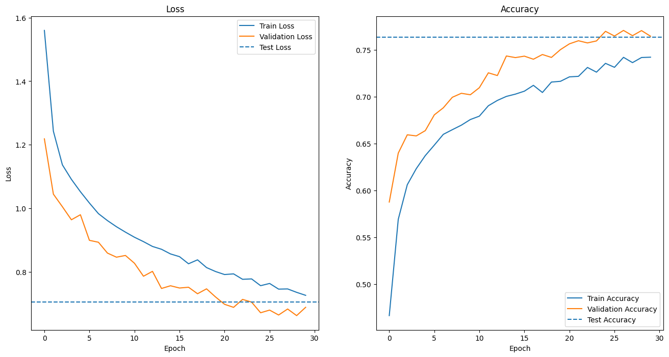
試作対応前のCNNモデルよりも精度が落ちたのは、中心クロップレイヤーを導入したことにより、背景画像に焦点の当たる割合が減った代わりに、全景画像に焦点の当たる割合が増えたためと推測します。
しかし、以下の画像が示す通り、中央クロップレイヤーを導入したことによって、前傾画像の葉に焦点を当てる目的は達成できました。


モデルによる予測
validフォルダのテスト用画像データを使用して、混同行列を可視化した結果は以下のようになりました。

各評価指数を以下に示します。
多値分類に対する評価指数ですので、マクロ平均値となります。
この結果を見る限り、多値分類のモデルとしての性能は良くありませんでした。
| 評価指数 | 値 |
|---|---|
| 正解率 | 0.7636 |
| マクロ平均適合性 | 0.7692 |
| マクロ平均再現性 | 0.7636 |
| マクロ平均F値 | 0.7609 |
そこで、「healthy」以外に分類される健康でない葉か「healthy」に分類される健康である葉かの2値分類として混同行列を作成すると、以下のようになります。
| 実際の値\予測値 | 健康でない | 健康 |
|---|---|---|
| 健康でない | 5600 | 278 |
| 健康 | 56 | 749 |
上記の混同行列から算出した評価指数は以下のようになります。
| 評価指数 | 値 |
|---|---|
| 正解率 | (5600 + 749) / 6683 = 0.8795 |
| 適合率 | 5600 / (5600 + 56) = 0.9901 |
| 再現率 | 5600 / (5600 + 278) = 0.9525 |
| F値 | 0.9710 |
この問題の課題は、葉の状態が健康でないことを認識することなので、健康でない葉のうち実際に健康でないと判定できたことを表す再現率で、モデルの性能が評価されるべきと考えます。
この視点でモデルを評価すると、再現率は0.9525と高い結果を示しましたが、適合率が再現率よりも高く、モデルの性能としては良い傾向とはなりませんでした。
作成したアプリ
構築したモデルでトマトの葉の画像を識別するアプリを、Renderにデプロイしました。トマトの葉の画像をアップロードしてお試しください。
次のステップ
データの前処理の工夫
AIが背景画像に着目しないように、背景画像を除去するためにRembgライブラリやOpenCVのGrabCutを試しましたが、どちらも処理に膨大な時間がかかり、採用することができませんでした。背景画像除去の高速化に取り組むことは興味深い課題です。
モデル構築
Kerasにはまだまだ多くの種類のレイヤーが定義されています。これらのレイヤーを利用して、再現率を向上させた最適なモデル構築に挑戦したいと考えています。
物体検出機構を実装して、葉の部分を確実に抽出する実装にも挑戦したいと考えています。
終わりに
AIアプリ開発の講座を通して、Pythonを使ったデータ分析から機械学習、ニューラルネットワークの学習を終えることができました。
在籍期間の残りを有効活用して、さらにスキルを磨いていき、より高度な課題のコンペに挑戦したり、さらに深い理解を得るように頑張ります。その過程で、新しいテクノロジーやツールにも積極的に触れていこうと思います。