検証環境
- MacOS Mojave 10.14.4
- Python 3.6.8
- numpy 1.15.0
- pandas 0.23.4
- matplotlib 2.2.2
- mpl-finance 0.10.0
OHLCデータ
OHLCデータは、Cryptowatchから取得したBTCFX/JPYの1分足データを使用しました。
https://api.cryptowat.ch/markets/bitflyer/btcfxjpy/ohlc?periods=60&after=1557172800&before=1557176340
import json
import requests
import datetime
import numpy as np
import matplotlib.dates as mdates
import matplotlib.pyplot as plt
from datetime import datetime, timedelta, timezone
from pandas import DataFrame, Series, to_datetime, concat
from mpl_finance import candlestick_ohlc

if __name__ == '__main__':
    response = json.loads(requests.get("https://api.cryptowat.ch/markets/bitflyer/btcfxjpy/ohlc?periods=60&after=1557172800&before=1557176340").text)

    # 7番目の要素はdocsに記載がないので何なのか不明
    df = pd.DataFrame(response['result']['60'], columns=['date','open','high','low','close','volume','unknown']).dropna().drop(columns=['volume','unknown'])
    # print(df.head(3))
    #         date    open    high     low   close
    # 0  1557432000  664434  665011  663901  664755
    # 1  1557432060  664826  664826  663800  663834
    # 2  1557432120  663834  664117  663723  664069

    # レスポンスのタイムスタンプがUnixTimestamp形式なのでdatetime型に変換し、pandas.DatetimeIndexを設定する
    df['date'] = pd.to_datetime(df['date'], unit='s', utc=True)
    df.set_index('date', inplace=True)
    df.index = df.index.tz_convert('Asia/Tokyo')
    # print(df.head(3))
    #                             open    high     low   close
    # date
    # 2019-05-10 05:00:00+09:00  664434  665011  663901  664755
    # 2019-05-10 05:01:00+09:00  664826  664826  663800  663834
    # 2019-05-10 05:02:00+09:00  663834  664117  663723  664069

    plt.style.use('ggplot')

    ax = plt.subplot()
    ax.xaxis.set_major_locator(mdates.AutoDateLocator())
    ax.xaxis.set_major_formatter(mdates.DateFormatter('%H:%M', tz=timezone(timedelta(hours=9))))

    # candlestick_ohlc の第二引数に渡すタプルイテレータを生成
    # @see https://github.com/matplotlib/mpl_finance/blob/master/mpl_finance.py
    quotes = zip(mdates.date2num(df.index), df['open'], df['high'], df['low'], df['close'])
    candlestick_ohlc(ax, quotes, width=(1/24/len(df))*0.7, colorup='g', colordown='r')

    plt.show()

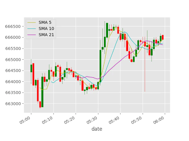
単純移動平均 (SMA)
def sma(ohlc: DataFrame, period=21) -> Series:
    return Series(
        ohlc['close'].rolling(period).mean(),
        name=f'SMA {period}',
    )
sma(df, 5).plot.line(color='y', legend=True)
sma(df, 10).plot.line(color='c', legend=True)
sma(df, 21).plot.line(color='m', legend=True)
指数平滑移動平均 (EMA)
def ema(ohlc: DataFrame, expo=21) -> Series:
    return Series(
        ohlc['close'].ewm(span=expo).mean(),
        name=f'EMA {expo}',
    )
ema(df, 5).plot.line(color='y', legend=True)
ema(df, 10).plot.line(color='c', legend=True)
ema(df, 21).plot.line(color='m', legend=True)

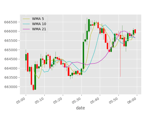
加重移動平均 (WMA)
def wma(ohlc: DataFrame, period: int = 9) -> Series:
    # WMA = ( 価格 * n + 価格(1) * n-1 + ... 価格(n-1) * 1) / ( n * (n+1) / 2 )
    denominator = (period * (period + 1)) / 2
    weights = Series(np.arange(1, period + 1)).iloc[::-1]

    return Series(
        ohlc['close'].rolling(period, min_periods=period).apply(lambda x: np.sum(weights * x) / denominator, raw=True),
        name=f'WMA {period}'
    )
wma(df, 5).plot.line(color='y', legend=True)
wma(df, 10).plot.line(color='c', legend=True)
wma(df, 21).plot.line(color='m', legend=True)
標準偏差
標準偏差
def sd(ohlc: DataFrame, period=10, ddof=0) -> float:
    return ohlc['close'].tail(period).std(ddof=ddof)
ddofは減算する自由度の数を示します。ddof=1を指定することで、不偏分散による標準偏差となります。
https://pandas.pydata.org/pandas-docs/stable/reference/api/pandas.Series.std.html
Delta Degrees of Freedom. The divisor used in calculations is N - ddof, where N represents the number of elements.
>>> sd(df, ddof=0)
232.7845570479279
>>> sd(df, ddof=1)
245.37646812828467