回答
図とコードが多くなりかなりスクロールする必要のある記事になったので、先に回答だけ示します。SciPyにあるVoronoiとDelaunayまたはConvexHullを組み合わせるとできます。後者は属性を表示するだけなので圧倒的に簡潔です。
from scipy.spatial import Voronoi, Delaunay, ConvexHull
import numpy as np
points = [(x0, y0, z0), (x1, y2, z2),...] # 原子位置
a, b, c = 5, 5, 5 # 格子定数
vor = Voronoi([(x*a, y*b, z*c) for x, y, z in points]) # Voronoi diagram計算
def CalcVolTetrahedron(a, b, c, d):
    tetravol = abs(np.dot((a-d), np.cross((b-d), (c-d))))/6
    return tetravol

def CalcVolVoronoiCell(vor, p):
    dpoints = []
    vol = 0
    for v in vor.regions[vor.point_region[p]]:
        # list of Voronoi indices (list of 3 integers) for Voronoi region 'p'
        dpoints.append(list(vor.vertices[v]))

    tri = Delaunay(np.array(dpoints))

    for simplex in tri.simplices:
        vol += CalcVolTetrahedron(np.array(dpoints[simplex[0]]),
                    np.array(dpoints[simplex[1]]),
                    np.array(dpoints[simplex[2]]),
                    np.array(dpoints[simplex[3]]))
    return vol

# pointsの先頭四つの原子のWS cellの体積を計算
for i, p in enumerate(vor.points[0:4]):
    pvol = CalcVolVoronoiCell(vor, i)
    print(f'point {i} with coordinates {np.round(p, 3)} has volume {pvol:.3f} A^3')
# pointsの先頭四つの原子のWS cellの体積を計算
pnts = [0, 1, 2, 3]

for p in pnts:
    ch = ConvexHull(vor.vertices[vor.regions[vor.point_region[p]]])
    print('volume:', ch.volume)
背景
うぃぐなーざいつせる?
結晶格子空間におけるWigner-Seitz cell(ウィグナーザイツセル)と波数空間におけるBrillouin zone(ブリリュアンゾーン)は固体物理の教科書の最初の方に出てくる似たような概念です。
| Wigner-Seitz cellの例 | Brillouin zoneの例 |
|---|---|
 By en:User:AndrewKepert CC BY-SA 3.0, Link |
.svg#/media/File:Brillouin_Zone_(1st,_FCC).svg) By Inductiveload Own work, Public Domain, Link |
どちらも「空間中のある点と周囲の点の垂直二等分面で囲まれる最小の領域」として定義されます。対象とする空間が実空間(軸の単位が長さ[$L$])か逆空間(単位が長さの逆数[$L^{-1}$])かという違いだけですが、必要になる場面が異なるため目にする頻度にもかなり差があります。例えばBrillouin zoneは物性の理解に必須なバンド構造を記述するのに欠かせない概念で物性系の論文では頻繁に出現しますが、演習問題の定番でもあるその体積が論文で言及されることはまずありません。一方、Wigner-Seitz cellはBrillouin zoneと一緒に教科書に出てきますが、論文で目にすること自体が少ないです。ただ、言及される場合はたいてい格子点の代わりに原子位置を使ったWigner-Seitz atomic cellの体積として出てきます1。
なんで体積がほしいの?
Brillouin zoneはもっぱら結晶構造の対称性と周期性が重要な場面で重宝されるため、研究者はその大きさや体積にあまり興味を持ちません。一方、Wigner-Seitz cell2は実際の結晶構造の中においてある原子位置に割り当てられた領域と解釈できるため、例えば大きさの異なる原子が結晶中のある位置に入り込みやすいかどうかなどを判定する際の目安として使えます。
体積計算なんてちょろくない?
私も「結晶構造が与えられればWigner-Seitz cellの体積なんて簡単に出せるでしょ」と思っていました。しかし、いざ計算する必要がでてきた際に「簡単な話だし誰かなんか作ってるっしょ」と色々調べてみた結果、「押すとWigner-Seitz cellの体積を計算してくれるボタンがついた道具」はどうやら存在しないことがわかりました3。
冒頭に挙げた図は面心立方格子の場合の非常に単純な例であり、綺麗な形をしているので体積の計算式も苦労せずに手計算で出せます。ところが、格子点ではなく原子位置を使ったWigner-Seitz cellの場合は単位格子中にたくさんの原子があるとかなり複雑な多面体を考える必要があり一筋縄では行きません。ところで、Wigner-Seitz cellもBrillouin zoneも固体物理学に登場する概念ですが、どちらも幾何学的にはVoronoi diagram(下図)と呼ばれるものです。Voronoi diagramは、区分けが必要な学問・実務領域で広く活用されているため、その大きさを評価する道具は絶対に揃っているはずです。

By Balu Ertl - Own work, CC BY-SA 4.0, Link
困った時のSciPy頼み
具体的な問題を数学的な固有名詞のついた問題のレベルまで落とし込めればSciPyがだいたい解決してくれます。調べてみると、予想通りVoronoi diagramを計算する関数がありました。
scipy.spatial.Voronoi — SciPy v1.1.0 Reference Guide
Voronoi diagramの頂点がわかれば、Delaunay triangulationを使って多面体を四面体要素に分割し、四面体の体積公式を使って求めた各要素の体積を足せば解決です4。これもSciPyにあります。
scipy.spatial.Delaunay — SciPy v1.1.0 Reference Guide
まさにこれです。
環境とパッケージ
Python 3.6, Jupyter notebookを使っています。
%matplotlib notebook # 3Dプロットをぐりぐり回せるnotebookにしました

from scipy.spatial import Voronoi, Delaunay, ConvexHull
import numpy as np
import matplotlib.pyplot as plt
import mpl_toolkits.mplot3d as a3
from scipy import __version__ as spv
from matplotlib._version import get_versions as mplv

print(mplv()['version']) #3.0.0
print(spv) # 1.1.0
print(np.__version__) # 1.13.3
対象とする物質と原子位置
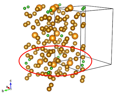
ネオジム磁石の主成分である強磁性体Nd2Fe14Bの結晶構造からc=0にある四つのNdのWigner-Seitz cellを計算しましょう5。この結晶構造には対称性の異なる2種類のNdサイトがあります。対称性が異なるので隣接する原子も異なり、必然的にWigner-Seitz cellの体積も違うはずです。そこで実際に二つのNdサイトの体積を求めてどれくらい違うか確かめてみましょう。まずはNdとその周辺にある原子(下図の赤線で囲った部分)の原子位置と格子定数を定義しておきます6。
a, b, c = 8.79212, 8.79212, 12.17789
points = [(1.14222, 0.85778, 0.00000), # Nd
          (0.85778, 1.14222, 0.00000), # Nd
          (1.27007, 1.27007, 0.00000), # Nd
          (0.72993, 0.72993, 0.00000), # Nd
          (0.96304, 0.64079, -0.176), # 以下しばらくFe
          (0.96304, 0.64079, 0.176),
          (0.64079, 0.96304, -0.176),
          (0.64079, 0.96304, 0.176),
          (1.03696, 1.35921, -0.176),
          (1.03696, 1.35921, 0.176),
          (1.35921, 1.03696, -0.176),
          (1.35921, 1.03696, 0.176),
          (1.22493, 0.56665, -0.12782),
          (1.22493, 0.56665, 0.12782),
          (1.22493, 1.56665, -0.12782),
          (1.22493, 1.56665, 0.12782),
          (0.43335, 0.77507, -0.12782),
          (0.43335, 0.77507, 0.12782),
          (1.43335, 0.77507, -0.12782),
          (1.43335, 0.77507, 0.12782),
          (1.56665, 1.22493, -0.12782),
          (1.56665, 1.22493, 0.12782),
          (0.56665, 1.22493, -0.12782),
          (0.56665, 1.22493, 0.12782),
          (0.77507, 1.43335, -0.12782),
          (0.77507, 1.43335, 0.12782),
          (0.77507, 0.43335, -0.12782),
          (0.77507, 0.43335, 0.12782),
          (0.90202, 0.90202, -0.20414),
          (0.90202, 0.90202, 0.20414),
          (1.09798, 1.09798, -0.20414),
          (1.09798, 1.09798, 0.20414),
          (1.183, 0.817, -0.25425),
          (1.183, 0.817, 0.25425),
          (1.317, 1.317, -0.24575),
          (1.317, 1.317, 0.24575),
          (0.817, 1.183, -0.25425),
          (0.817, 1.183, 0.25425),
          (0.68306, 0.68306, -0.24575),
          (0.68306, 0.68306, 0.24575),
          (0.50000, 0.50000, -0.11500),
          (0.50000, 0.50000, 0.11500),
          (1.50000, 1.50000, -0.11500),
          (1.50000, 1.50000, 0.11500),
          (0.50000, 1.00000, 0.00000),
          (0.50000, 1.00000, 0.00000),
          (1.00000, 0.50000, 0.00000),
          (1.50000, 1.00000, 0.00000),
          (1.00000, 1.50000, 0.00000),
          (1.50000, 1.00000, 0.00000),
          (1.00000, 0.50000, 0.00000),
          (1.00000, 1.50000, 0.00000),
          (0.62347, 0.37653, 0.00000), # 以下B
          (0.37653, 0.62347, 0.00000),
          (0.62347, 1.37653, 0.00000),
          (1.37653, 1.62347, 0.00000),
          (1.62347, 1.37653, 0.00000),
          (1.37653, 0.62347,0.00000)]
原子が多いのでかなり長大なリストになりますが、どうやって作ったかは忘れました。VESTAでぽちぽちクリックしたのかもしれません。
まずはSciPyのVoronoiオブジェクトを理解する
import antigravityで空に浮かんでPCに手が届かなくなる前に地上への降り方をあらかじめ調べておきましょう。SciPyの公式ドキュメントを見ると、属性にverticesやridgeといった耳慣れない単語があります。これらはVoronoi diagramを扱う上で必須の重要な情報なのですが、かなり関係が入り組んでいるためコードを書いてるうちに簡単に迷子になります。幸いなことに、Qiitaのこちらの記事に大変わかりやすい図解があったので、以下はこの図と照らし合わせながら読んでいくと理解が早いと思います。
Voronoiオブジェクトの属性の可視化
Voronoiオブジェクトの各属性がどんなものか、それぞれ最初の3点だけちょっと見てみましょう。注意すべきはある点についての情報が結晶構造中での座標(coordinate)なのか、点を保持したリストの中での位置を示すインデックスなのかです。
# 後ほど求める体積が正しい値になるように格子定数を掛ける
vor = Voronoi([(x*a, y*b, z*c) for x, y, z in points])

# 入力に使った原子位置(格子定数をかける前の値)
print(f'atomic positions\nshape={np.array(points).shape}')
print(points[:3], '\n')

# vorが保持している入力された原子位置(格子定数をかけた後の値)
print(f'vor.points in coordinate\nshape={vor.points.shape}')
print(vor.points[:3], '\n')

# 入力点から計算した全てのVoronoi regionの頂点(vertex、複数形はvertices)の座標
print(f'vor.vertices in coordinate\nshape={vor.vertices.shape}')
print(vor.vertices[:3], '\n')

# ridge(2Dは垂直二等分線、3Dは垂直二等分面)を求める際に使った二つの入力点のインデックス
print(f'vor.ridge_points in "point" index\nshape={vor.ridge_points.shape}')
print(vor.ridge_points[:3], '\n')

# 上の二点を座標で表示
print(f'vor.ridge_points in coordinate')
print(vor.points[vor.ridge_points][:3], '\n')

# ridgeを構成する頂点のvor.verticesにおけるインデックス
# -1はVoronoi diagramの外側
print(f'vor.ridge_vertices in "vertex" index\nlength={len(vor.ridge_vertices)}')
print('-1 represents a point outside of the Voronoi diagram')
print(np.array(vor.ridge_vertices)[:3], '\n')

# 上のverticesを座標で表示
# -1はvor.verticesの最後の要素を表示してしまう点に注意
print("vor.ridge_vertices in cordinates")
print('Note that -1 in index gives the last element of a list or numpy array.')
for i in np.array(vor.ridge_vertices)[:3]:
    print(vor.vertices[i])
print('\n')

# Voronoi regionの多面体を構成する頂点のvor.verticesにおけるインデックス
print(f'vor.regions in "vertex" index\nlength={len(vor.regions)}')
print(vor.regions[:3], '\n')

# vor.pointsの各入力点が属するVoronoi regionを示すvor.regionsにおけるインデックス
print(f'vor.point_region in "region" index\nshape={vor.point_region.shape}')
print(vor.point_region[:3], '\n')

# 8番目の入力点での例
print('Example')
print('The coordinate of eighth point is, ') # 8番目の入力点の座標
print('vor.points[7]=', vor.points[7], '\n')
print('This point is in a Voronoi region,') # この点が属するVoronoi region
print('vor.point_region[7]=', vor.point_region[7], '\n')
print('This region is formed by these Voronoi vertices,') # そのVoronoi regionを構成する頂点のインデックス
print('vor.regions[vor.point_region[7]]=', vor.regions[vor.point_region[7]], '\n')
print('The coordinates of the vertices are,') # その頂点の座標
print('vor.vertices[vor.regions[vor.point_region[7]]]=', vor.vertices[vor.regions[vor.point_region[7]]], '\n')
atomic positions
shape=(58, 3)
[(1.14222, 0.85778, 0.0), (0.85778, 1.14222, 0.0), (1.27007, 1.27007, 0.0)]

vor.points in coordinate
shape=(58, 3)
[[ 10.04253531   7.54170469   0.        ]
 [  7.54170469  10.04253531   0.        ]
 [ 11.16660785  11.16660785   0.        ]]

vor.vertices in coordinate
shape=(173, 3)
[[  9.82700359e+00   9.82700359e+00   8.73907706e+00]
 [ -4.83532814e+14  -4.83532814e+14   0.00000000e+00]
 [  1.89847783e+01   7.49633631e+00   1.39889465e+01]]

vor.ridge_points in "point" index
shape=(257, 2)
[[41 52]
 [41 53]
 [41 27]]

vor.ridge_points in coordinate
[[[ 4.39606     4.39606     1.40045735]
  [ 5.48162306  3.31049694  0.        ]]

 [[ 4.39606     4.39606     1.40045735]
  [ 3.31049694  5.48162306  0.        ]]

 [[ 4.39606     4.39606     1.40045735]
  [ 6.81450845  3.8100652   1.5565779 ]]]

vor.ridge_vertices in "vertex" index
length=257
-1 represents a point outside of the Voronoi diagram
[list([-1, 1, 15, 14]) list([-1, 1, 9, 8]) list([-1, 14, 11])]

vor.ridge_vertices in cordinates
Note that -1 in index gives the last element of a list or numpy array.
[[ -2.59158034e+01   1.24622879e+02   5.17124623e-16]
 [ -4.83532814e+14  -4.83532814e+14   0.00000000e+00]
 [  5.25540998e+00   5.07319417e+00  -2.88992138e-16]
 [  5.85323103e+00   4.89310354e+00   6.02997430e-01]]
[[ -2.59158034e+01   1.24622879e+02   5.17124623e-16]
 [ -4.83532814e+14  -4.83532814e+14   0.00000000e+00]
 [  5.07319417e+00   5.25540998e+00  -2.88992138e-16]
 [  4.89310354e+00   5.85323103e+00   6.02997430e-01]]
[[ -2.59158034e+01   1.24622879e+02   5.17124623e-16]
 [  5.85323103e+00   4.89310354e+00   6.02997430e-01]
 [  5.91412643e+00   5.33952874e+00   1.33531905e+00]]


vor.regions in "vertex" index
length=55
[[-1, 1, 8, 9, 11, 12, 14, 15], [-1, 1, 9, 10, 15, 16, 17, 18], [-1, 32, 33, 35, 36, 39, 40]]

vor.point_region in "region" index
shape=(58,)
[29 48 47]

Example
The coordinate of eighth point is,
vor.points[7]= [ 5.63390257  8.46716324  2.14330864]

This point is in a Voronoi region,
vor.point_region[7]= 37

This region is formed by these Voronoi vertices,
vor.regions[vor.point_region[7]]= [41, 42, 43, 44, 45, 46, 47, 48, 145, 147, 151, 153]

The coordinates of the vertices are,
vor.vertices[vor.regions[vor.point_region[7]]]= [[  5.57299549   6.82827784   1.49334209]
 [  6.60938318   7.0442508    1.6657878 ]
 [ -1.40028323  10.08742334  13.9895067 ]
 [ -1.66633821  10.58849594  13.40515171]
 [  6.36015961   8.21598693   5.17056905]
 [  7.02722273   8.21533727   0.69872926]
 [  6.54682828   9.87831886   1.49344317]
 [  7.14917195   9.33013273   1.6266743 ]
 [  6.36505971   8.42067221   0.26024968]
 [  5.93758435   9.4960634    0.67017797]
 [  5.23531638   7.45884052   0.76689192]
 [  3.28576674   9.12111589   2.14485639]]
この出力を見ても想像がつかないので可視化します。
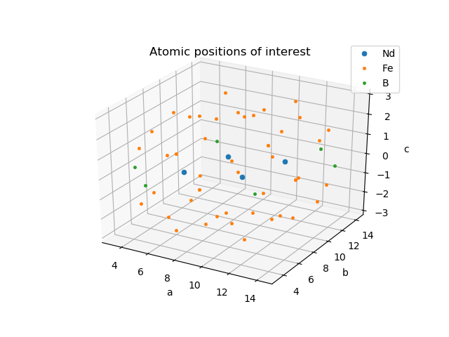
points
fig = plt.figure()
ax = fig.add_subplot(111, projection='3d')

ax.set_xlabel('a')
ax.set_ylabel('b')
ax.set_zlabel('c')
ax.set_title('Atomic positions of interest')
x, y, z = vor.points[:, 0], vor.points[:, 1], vor.points[:, 2]
ax.plot(x[0:4,], y[0:4], z[0:4], "o", ms=5, mew=0.5, label='Nd')
ax.plot(x[4:-6], y[4:-6], z[4:-6], "o", ms=3, mew=0.5, label='Fe')
ax.plot(x[-6:], y[-6:], z[-6:], "o", ms=3, mew=0.5, label='B')
ax.legend()
これは説明もいらないでしょう。入力点の座標です。先に示した結晶構造の赤線で囲んだ部分の原子だけが表示されています。
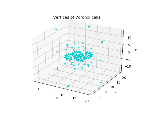
vertices
fig = plt.figure()
ax = fig.add_subplot(111, projection='3d')

ax.set_xlabel('a')
ax.set_ylabel('b')
ax.set_zlabel('c')
ax.set_title('Vertices of Voronoi cells')
x, y, z = vor.vertices[:, 0], vor.vertices[:, 1], vor.vertices[:, 2]
# excluding vertices too far from ROI
roi = (np.abs(x) < 20) & (np.abs(y) < 20)
ax.plot(x[roi], y[roi], z[roi], "o", color="#00cccc", ms=4, mew=0.5)
複雑な多面体の頂点が全てプロットされているのでこれだけでは何が何だかわかりません。
ridge_points
fig = plt.figure()
ax = fig.add_subplot(111, projection='3d')

ax.set_xlabel('a')
ax.set_ylabel('b')
ax.set_zlabel('c')
ax.set_title('Pairs of atoms between which each Voronoi ridge plane lies')
for pair in vor.points[vor.ridge_points]:
    ax.plot(pair[:, 0], pair[:, 1], pair[:, 2], color='C0')
多面体の面を垂直に貫く二点を結ぶ全ての線がまとめて表示されています。これも何が何だかわかりません。
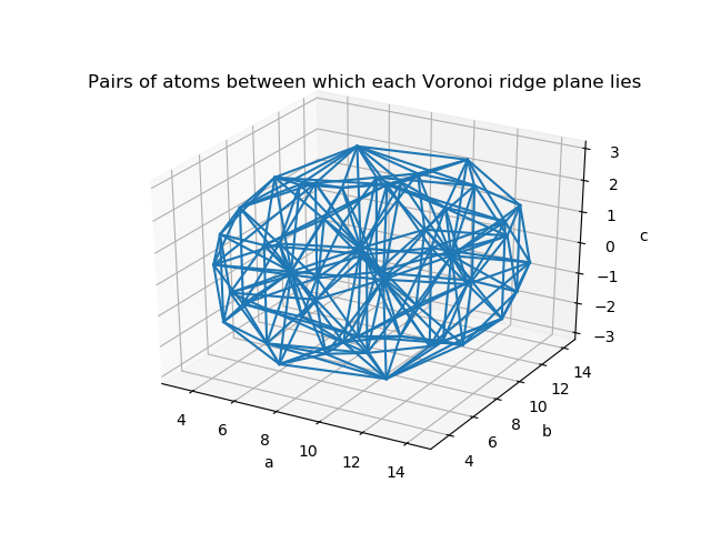
fig = plt.figure()
ax = fig.add_subplot(111, projection='3d')
ax.set_xlabel('a')
ax.set_ylabel('b')
ax.set_zlabel('c')
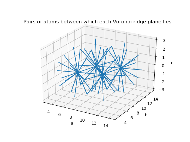
ax.set_title('Pairs of atoms between which each Voronoi ridge plane lies')
for pair, pair_index in zip(vor.points[vor.ridge_points], vor.ridge_points):
if np.any([i in list(pair_index) for i in [0, 1, 2, 3]]):
ax.plot(pair[:, 0], pair[:, 1], pair[:, 2], color='C0')
一端がNdである線だけに限定すると、様子がわかってきます。線が集中している四点にNdがあり、各線分のもう一端にNdに隣接する各原子があります。
ridge_vertices
fig = plt.figure()
ax = fig.add_subplot(111, projection='3d')
ax.set_xlabel('a')
ax.set_ylabel('b')
ax.set_zlabel('c')
ax.set_aspect('equal')
ax.set_xlim(3, 15)
ax.set_ylim(3, 15)
ax.set_zlim(-6, 6)
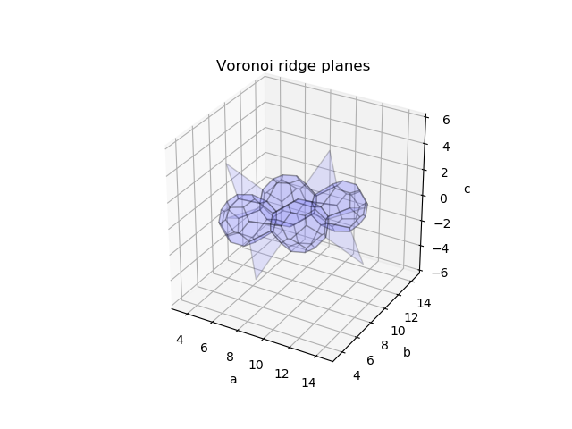
ax.set_title('Voronoi ridge planes')
ridgenum = 0
for i in np.array(vor.ridge_vertices):
# exclude ridge planes with points outside ROI
if -1 not in i:
vertices = vor.vertices[i]
# only display ridge planes which fit within -3<c<3
# This will show some planes which don't belong to Voronoi regions of Nd sites
xy, z = vertices[:, :-1], vertices[:, -1]
if (xy.min() > 3) & (xy.max() < 15) & (np.abs(z).max() < 3):
ridgenum += 1
poly=a3.art3d.Poly3DCollection([vertices],alpha=0.2)
poly.set_edgecolor('k')
poly.set_facecolor([0.5, 0.5, 1])
ax.add_collection3d(poly)
print('No. of all ridge planes:', len(vor.ridge_vertices))
print('No. of ridge planes displayed:', ridgenum)
# No. of all ridge planes: 257
# No. of ridge planes displayed: 83
入力点の垂直二等分面を表示しています。異常に大きな面を排除して表示するとNdのWigner-Seitz cellに相当するVoronoi領域が見えましたが、余計な面が混ざっています。
regionsとpoint_region
fig = plt.figure()
ax = fig.add_subplot(111, projection='3d')
ax.set_xlabel('a')
ax.set_ylabel('b')
ax.set_zlabel('c')
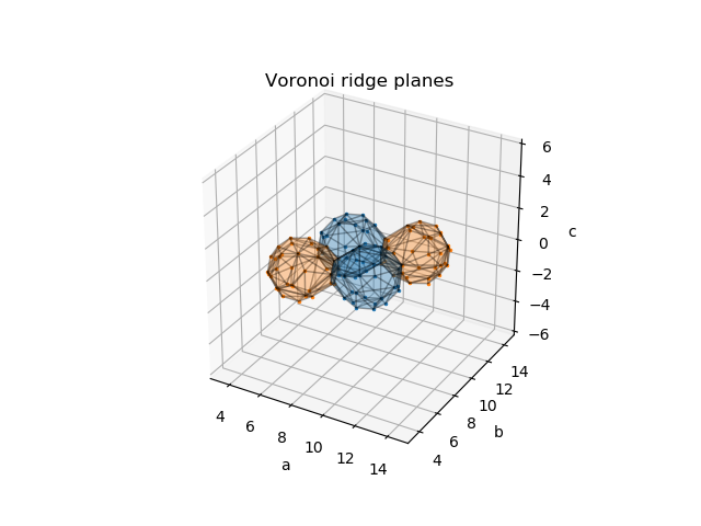
ax.set_title('Voronoi ridge planes')
pnts = [0, 1, 2, 3] # Nd sites
for p in pnts:
color = f'C{p//2}' # 'C0' or 'C1'
# Voronoi regionの頂点から凸包(convex hull)を求めてその面を表示
ch = ConvexHull(vor.vertices[vor.regions[vor.point_region[p]]])
poly = a3.art3d.Poly3DCollection(ch.points[ch.simplices], alpha=0.2, facecolor=color, edgecolor='k')
ax.add_collection3d(poly)
chpnts = ch.points[ch.vertices]
ax.plot(chpnts[:, 0], chpnts[:, 1], chpnts[:, 2], ".", color=color, ms=4, mew=0.5)
ax.set_aspect('equal')
ax.set_xlim(3,15)
ax.set_ylim(3,15)
ax.set_zlim(-6,6)
Ndの原子位置のVoronoi regionだけを表示させるとWigner-Seitz cellが表示できました。
SciPyのDelaunayを使って体積を求める
3次元のDelaunay triangulationは多面体を四面体に分割してくれます。四面体の体積計算には非常に簡単な公式を使えるので、各四面体の体積を足せばVoronoi cellの体積が求まります。StackOverflowのこの回答を参考にした以下のコードで計算します。
def CalcVolTetrahedron(a, b, c, d):
    '''
    Calculates the volume of a tetrahedron with vertices a,b,c and d
    a, b, c, d: tuples of (x, y, z)
    '''

    tetravol = abs(np.dot((a-d), np.cross((b-d), (c-d))))/6
    return tetravol

def CalcVolVoronoiCell(vor, p):
    '''
    Calculate the volume of a 3D Voronoi cell.
    vor: a Voronoi diagram object returned by scipy.spatial.Voronoi.
    p: the index number of vor to specify Voronoi cell
    '''

    dpoints = []
    vol = 0
    for v in vor.regions[vor.point_region[p]]:
        # list of Voronoi indices (list of 3 integers) for Voronoi region 'p'
        dpoints.append(list(vor.vertices[v]))

    tri = Delaunay(np.array(dpoints))

    for simplex in tri.simplices:
        vol += CalcVolTetrahedron(np.array(dpoints[simplex[0]]),
                    np.array(dpoints[simplex[1]]),
                    np.array(dpoints[simplex[2]]),
                    np.array(dpoints[simplex[3]]))
    return vol

for i, p in enumerate(vor.points[0:4]):
    # vor.regions includes -1 if one of vertices is outside the ROI.
    # In our case, this can be ignored.
    if -1 in vor.regions[vor.point_region[i]]:
        out = True
    else:
        out = False

    if not out:
        pvol = CalcVolVoronoiCell(vor, i)
        print(f'point {i} with coordinates {np.round(p, 3)} has volume {pvol:.3f} A^3')

# point 0 with coordinates [ 10.043   7.542   0.   ] has volume 22.162 A^3
# point 1 with coordinates [  7.542  10.043   0.   ] has volume 22.162 A^3
# point 2 with coordinates [ 11.167  11.167   0.   ] has volume 20.147 A^3
# point 3 with coordinates [ 6.418  6.418  0.   ] has volume 20.147 A^3
2種類のNdサイトの体積の差が定量的にわかりました。ようやく目的達成です。
実はSciPyのConvexHullで一発だった
この問題に遭遇した当時は上の方法を使って一件落着したのですが、後日調べたらSciPyのConvexHullにvolumeというドンピシャの属性があるのを見つけました。おそらく当時(数年前)はまだ実装されていなかったものです。
pnts = [0, 1, 2, 3] # Nd sites

for p in pnts:
    ch = ConvexHull(vor.vertices[vor.regions[vor.point_region[p]]])
    print('volume:', ch.volume)
# volume: 22.161550294014237
# volume: 22.161550294014233
# volume: 20.146904864244863
# volume: 20.146604828322054
当然ながら、Delaunay triangulationを使って求めた値と一致しています。今後使うならこれですね。
Wigner-Seitz cellをVESTAで表示する
ここまではmatplotlibを使って可視化してきましたが、結晶構造の可視化はやはりVESTAが一番です7。
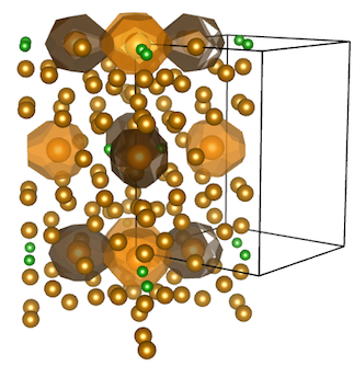
上の図を作った時の詳しい手順は失念してしまいましたが、以下のような感じだったと思います。
- 凸包の頂点に仮想的に原子があることにしてCIFファイルに追記
- Wigner Seitz cellの中にある原子と仮想原子のBondを表示する(原子間距離の範囲はうまく調整)。
- ObjectsタブのVのチェックを外して仮想原子を非表示に
- Polygon表示モードにする
CIFファイルに追記する仮想原子のリストは以下で生成できます。
pnts = [0, 1, 2, 3] # Nd sites
# assign different elements to different sites
els = ['H', 'H', 'He', 'He']

for p, el in zip(pnts, els):
    ch = ConvexHull(vor.vertices[vor.regions[vor.point_region[p]]])
    chpnts = ch.points[ch.vertices]
    normalizer = np.tile(np.array([a, b, c]), (len(chpnts), 1))
    chpnts = chpnts/normalizer
    print(f'# point {p}')
    for x, y, z in chpnts:
        print(f' {el} {x:.4f} {y:.4f} {z:.4f} 0.1 1.000 Uiso {el}')
# point 0
 H 1.1869 0.9388 0.1336 0.1 1.000 Uiso H
 H 1.2554 0.8765 0.1226 0.1 1.000 Uiso H
 H 1.3442 0.8254 -0.0000 0.1 1.000 Uiso H
 H 1.2007 1.0656 -0.0574 0.1 1.000 Uiso H
 H 1.2007 1.0656 0.0574 0.1 1.000 Uiso H
 H 1.0888 0.9112 0.1395 0.1 1.000 Uiso H
 H 1.2307 0.7693 0.1157 0.1 1.000 Uiso H
 H 1.2594 0.7406 0.0721 0.1 1.000 Uiso H
...
...
-
Wigner-Seitz cellの本来の定義では格子点を使っていますが、研究の現場ではより使い道のある原子位置をベースにしたWigner-Seitz atomic cellが置換系における原子半径とサイト占有率を論じる際などに使われます。 ↩
-
本稿ではatomic cellのみを扱うので以降はatomicを省略してWigner-Seitz cellと表記します。 ↩
-
ただし、ググっても出てこないようなちょっとした便利機能としてなんらかのソフトに実装されている可能性は高いです。何か知っていたら教えてください。 ↩
-
さもDelaunay triangulationを知っていたかのように書いていますが、のちほど紹介するStack Overflowの回答を見て初めて知りました。 ↩
-
簡単な構造だと張り合いがないのでいきなり単位格子内の原子数が多い例でやってみます。 ↩
-
単位格子から少しずれた場所を使っているのは、確か互いに接しているようなNdのWigner-Seitz cellを求めたかったからです。理由は忘れました。 ↩
-
面が描画されておらず妙な隙間のできてるPolygonがありますが、原因はよくわかりません。 ↩