Pythonで理解する物理のエッセンス 熱・電磁気・原子 (河合塾シリーズ)

解説動画が豊富

p13分子の平均運動エネルギー

import numpy as np
import matplotlib.pyplot as plt

# ボルツマン定数 (J/K)
k = 1.38e-23

# 温度の範囲を設定します (0から1000K)
temperature_range = np.linspace(0, 1000, 1000)

# 平均運動エネルギーを計算します
average_energy = 1.5 * k * temperature_range

# グラフをプロットします
plt.figure(figsize=(8, 6))
plt.plot(temperature_range, average_energy, label='Average Energy')
plt.xlabel('Temperature (K)')
plt.ylabel('Average Energy (J)')
plt.title('Average Kinetic Energy of Molecules vs Temperature')
plt.legend()
plt.grid(True)
plt.show()

結果

p22
断熱変化の式

import numpy as np
import matplotlib.pyplot as plt

# 定数の設定
gamma = 1.4  # 比熱比

# プロットする範囲の定義
V = np.linspace(0.1, 10, 100)  # 体積の範囲を設定
T_const = 1  # 一定の温度

# TV^(gamma - 1) = constの式からTを求める
T = T_const / V**(gamma - 1)

# グラフのプロット
plt.plot(V, T)
plt.xlabel('Volume (V)')
plt.ylabel('Temperature (T)')
plt.title('Adiabatic Process: TV^(gamma-1) = const')
plt.grid(True)
plt.show()

結果

import numpy as np
import matplotlib.pyplot as plt

def calculate_capacitance(epsilon, area, distance):
    capacitance = epsilon * area / distance
    return capacitance

コンデンサーの誘電率
# 誘電率（F/m）
epsilon = 8.854e-12  # 真空の誘電率を示す

# 極板間の距離（m）
distance_values = np.linspace(0.001, 0.1, 100)

# 極板間の面積（m^2）
area_values = [0.01, 0.02, 0.03]

plt.figure(figsize=(10, 6))

for area in area_values:
    capacitance_values = [calculate_capacitance(epsilon, area, d) for d in distance_values]
    plt.plot(distance_values, capacitance_values, label=f'Area = {area} m^2')

plt.xlabel('Distance (m)')
plt.ylabel('Capacitance (F)')
plt.title('Capacitance vs Distance for Different Areas')
plt.legend()
plt.grid(True)
plt.show()

結果

p61
1次遅れ系微分方程式
Ty’(t)+y(t)＝K
初期条件Kのとき
y(t)=K(1-exp(-t/T)
Tは時定数
Kはゲイン

import sympy as sp
import numpy as np
import matplotlib.pyplot as plt

# 変数の定義
t = sp.symbols('t')
y = sp.Function('y')(t)

# 定数の定義
T, K, y0 = sp.symbols('T K y0')

# 初期条件の定義
initial_conditions = {y.subs(t, 0): y0}

# 微分方程式の定義
diff_eq = sp.Eq(T * sp.diff(y, t) + y, K)

# 初期条件を考慮して微分方程式を解く
solution_with_initial_conditions = sp.dsolve(diff_eq, y, ics=initial_conditions)

# 解の式を取得
solution_expr = solution_with_initial_conditions.rhs

# 解の式をラムダ関数に変換
y_func = sp.lambdify((t, T, K, y0), solution_expr, 'numpy')

# パラメータの値を設定
T_val = 1  # Tの値
K_val = 1  # Kの値
y0_val = 0  # y(0)の値

# 時刻の範囲を設定
t_values = np.linspace(0, 10, 100)

# 解を評価してプロット
y_values = y_func(t_values, T_val, K_val, y0_val)

plt.plot(t_values, y_values)
plt.xlabel('Time')
plt.ylabel('y(t)')
plt.title('Solution of the differential equation')
plt.grid(True)
plt.show()

結果

p89
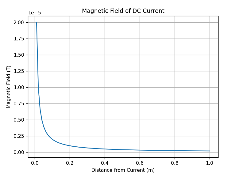
電流が作る磁場
直流電流
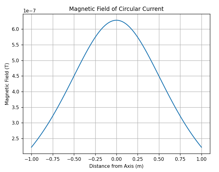
円形電流
ソレノイド

import numpy as np
import matplotlib.pyplot as plt

# 直流電流による磁場の強さを計算する関数
def calculate_dc_magnetic_field(I, r):
    mu_0 = 4 * np.pi * 10**-7  # 真空の透磁率
    return (mu_0 * I) / (2 * np.pi * r)

# 円形電流による磁場の強さを計算する関数
def calculate_circular_magnetic_field(I, R, z):
    mu_0 = 4 * np.pi * 10**-7  # 真空の透磁率
    return (mu_0 * I * R**2) / (2 * (R**2 + z**2)**(3/2))

# ソレノイドによる磁場の強さを計算する関数
def calculate_solenoid_magnetic_field(I, n):
    mu_0 = 4 * np.pi * 10**-7  # 真空の透磁率
    return mu_0 * n * I

# プロット範囲を設定
r_values = np.linspace(0.01, 1, 100)  # 直流電流の場合の距離
z_values = np.linspace(-1, 1, 100)    # 円形電流の場合の距離

# 直流電流による磁場のプロット
I_dc = 1  # 直流電流の強さ
B_dc = [calculate_dc_magnetic_field(I_dc, r) for r in r_values]
plt.figure()
plt.plot(r_values, B_dc)
plt.title('Magnetic Field of DC Current')
plt.xlabel('Distance from Current (m)')
plt.ylabel('Magnetic Field (T)')
plt.grid(True)
plt.show()

# 円形電流による磁場のプロット
I_circular = 1  # 円形電流の強さ
R_circular = 1  # 円の半径
B_circular = [calculate_circular_magnetic_field(I_circular, R_circular, z) for z in z_values]
plt.figure()
plt.plot(z_values, B_circular)
plt.title('Magnetic Field of Circular Current')
plt.xlabel('Distance from Axis (m)')
plt.ylabel('Magnetic Field (T)')
plt.grid(True)
plt.show()

# ソレノイドによる磁場のプロット
I_solenoid = 1  # ソレノイドの電流の強さ
n_solenoid = 10  # ソレノイドの巻数密度
B_solenoid = calculate_solenoid_magnetic_field(I_solenoid, n_solenoid)
print("Magnetic Field of Solenoid:", B_solenoid, "T")
結果
![image.png](https://qiita-image-store.s3.ap-northeast-1.amazonaws.com/0/3760770/3c3d7705-d7f3-8d2c-3ba6-3e8434fba7fa.png)
![image.png](https://qiita-image-store.s3.ap-northeast-1.amazonaws.com/0/3760770/2ce62506-6fbf-b2d5-0f15-b44d7b4a4f96.png)


import numpy as np
import matplotlib.pyplot as plt

# 直流電流の磁場計算式
def calc_b_dc(I, r):
    mu_0 = 4 * np.pi * 1e-7
    return mu_0 * I / (2 * np.pi * r)

# 円形電流の磁場計算式
def calc_b_circle(I, R, z):
    mu_0 = 4 * np.pi * 1e-7
    return mu_0 * I * R**2 / (2 * (R**2 + z**2)**(3/2))

# ソレノイドの磁場計算式
def calc_b_solenoid(I, n):
    mu_0 = 4 * np.pi * 1e-7
    return mu_0 * n * I

# 電流の範囲とステップサイズ
I_values = np.linspace(0.1, 10, 100)

# 直流電流の場合
r = 1
B_dc = [calc_b_dc(I, r) for I in I_values]

# 円形電流の場合
R = 1
z = 1
B_circle = [calc_b_circle(I, R, z) for I in I_values]

# ソレノイドの場合
n = 1
B_solenoid = [calc_b_solenoid(I, n) for I in I_values]

# プロット
plt.figure(figsize=(10, 6))
plt.plot(I_values, B_dc, label='Direct Current')
plt.plot(I_values, B_circle, label='Circular Current')
plt.plot(I_values, B_solenoid, label='Solenoid')
plt.xlabel('Current (A)')
plt.ylabel('Magnetic Field (T)')
plt.title('Magnetic Field as a Function of Current')
plt.legend()
plt.grid(True)
plt.show()

結果

交流

シミュレーションできるサイト

ローレンツ力

import numpy as np
import matplotlib.pyplot as plt
from mpl_toolkits.mplot3d import Axes3D

# 電荷量
q = 1

# 原点での速度ベクトル
v = np.array([1, 1, 1])

# 原点での磁場ベクトル
B = np.array([0, 0, 1])  # z軸方向の磁場

# 原点でのローレンツ力の計算
F = q * np.cross(v, B)

# プロット用のデータ
origin = np.zeros(3)

# 三次元プロット
fig = plt.figure()
ax = fig.add_subplot(111, projection='3d')
ax.quiver(*origin, *v, color='r', label='Velocity')
ax.quiver(*origin, *B, color='g', label='Magnetic Field')
ax.quiver(*origin, *F, color='b', label='Lorentz Force')
ax.set_xlim([-1, 1])
ax.set_ylim([-1, 1])
ax.set_zlim([0, 1])
ax.set_xlabel('X')
ax.set_ylabel('Y')
ax.set_zlabel('Z')
ax.legend()
plt.show()

結果

p97
ファラデーの電磁誘導の法則

import numpy as np
import matplotlib.pyplot as plt

# パラメータ設定
N = 1  # コイルの巻き数

# 入力関数
def input_function(t):
    return np.sin(t)

# 入力関数の微分
def input_derivative(t):
    return np.cos(t)

# 出力関数
def output_function(t):
    return -N * input_derivative(t)

# 時間の範囲を設定
t = np.linspace(0, 10, 1000)

# 入力と出力の計算
input_signal = input_function(t)
output_signal = output_function(t)

# プロット
plt.figure(figsize=(10, 5))
plt.plot(t, input_signal, label='Input (Φ(t)) = sin(t)')
plt.plot(t, output_signal, label='Output (V(t)) = -N * dΦ/dt')
plt.xlabel('Time')
plt.ylabel('Signal')
plt.title('Input and Output Signals')
plt.legend()
plt.grid(True)
plt.show()

結果

import matplotlib.pyplot as plt

# 与えられた点の座標
points = {
    "Point 1": (0, 0),
    "Point 2": (R, 0),  # ここでRの値を指定する必要があります
    "Point 3": (0, omega * L - 1 / (omega * C)),  # ここでomega、L、Cの値を指定する必要があります
    "Point 4": (R, omega * L - 1 / (omega * C))  # ここでR、omega、L、Cの値を指定する必要があります
}

# 点の座標を抽出
x_values = [point[0] for point in points.values()]
y_values = [point[1] for point in points.values()]

# プロット
plt.scatter(x_values, y_values)

# ラベル付け
for label, (x, y) in points.items():
    plt.text(x, y, f'{label} ({x}, {y})')

# グラフの装飾
plt.xlabel('Real')
plt.ylabel('Imaginary')
plt.title('Complex Plane')

# グリッドを表示
plt.grid(True)

# 表示
plt.show()

結果

p134
ドブロイ波の式

import numpy as np
import matplotlib.pyplot as plt

# プランク定数
h = 6.62607015e-34  # m^2 kg / s

# 運動量の範囲を定義する
p_values = np.linspace(0, 1e-24, 1000)  # Adjust the range of momentum as needed

# ド・ブロイの波動方程式に従って波長を計算
wavelengths = h / p_values

# 表示
plt.plot(p_values, wavelengths)
plt.xlabel('Momentum (kg m/s)')
plt.ylabel('Wavelength (m)')
plt.title("de Broglie's Wave Relation")
plt.grid(True)
plt.show()