概要と背景
概要
- この記事では、深層強化学習のエージェント実装時に必要になる、数学的な計算処理の実装をいくつか紹介します
- この記事のメインは、連続行動空間における強化学習エージェントの学習において Advantage を利用する際に必要になる、Action の対数確率密度 (log-probability density) を計算する方法についての解説です
背景
- 強化学習のコードを書いていると、log、exp、正規分布、tanh、対数確率密度 (log_prob) などを用いた複雑な数式が現れることがある。
- 自分の場合、これらの実装が正しいのかどうかを確認する術がなくて困った。
- そこで、「よく使われる計算については実装してコードを記録しておこう」と思い立ち、この記事を書くことにしました。
題材
いずれも、「数式上はそういう結果になる」ということはわかっているものの、**「数式と実装とが合っているのか」**については確信が持てないものを題材とした。
数式の通りに実装したつもりであっても、実はその実装は数式を正しく反映していないということはよくある。その可能性を潰すために、このような確認を行った。
①初めのいっぽ (^ワ^*)
最初は非常に単純な動作確認。小手調べ。
②標準的な処理
ほんの少し実用的。ちゃんと期待通りに動いているのか、ちょっと気になる処理。
- 3.1次元正規分布からデータをサンプリングする
- 4.
多次元正規分布からデータをサンプリングする(未対応)
③応用: 対数確率密度 (log_probs / log_pis) の計算
分布関数からサンプリングされた行動 (Action) の対数確率密度を計算する。
この記事を書く前は、対数確率密度の計算で何が行われているのか一見してよくわからなかった。しかし、数式を確認したり、 pytorch に実装されているコードも見たりして、何とか理解できたので記事にした。
-
- 5-1. Action を単純に正規分布からサンプリング
- 5-2. Action を出力する際に、正規分布からサンプリングした値を
tanh関数に通して Action とする
-
6.多次元正規分布からサンプリングしている場合
正しく実装するのはとても大変だった。- 6-1. Action を単純に正規分布からサンプリング
- 6-2. Action を出力する際に、正規分布からサンプリングした値を
tanh関数に通して Action とする - 6-3. Action を出力する際に、正規分布からサンプリングした値を
tanh関数に通し、その上で scaling を行って Action とする
これら①②③の動作確認を行う。
動作環境
| item | version |
|---|---|
| OS | google colaboratory |
| Python | 3.11.11 |
| torch | 2.6.0+cu124 |
ソースコードと確認結果
「5.」以降のソースコードは、github にもアップロードしています1。
0. モジュールのインポート
import math

from matplotlib import pyplot as plt
import numpy as np
import pandas as pd

import torch
from torch.distributions import Normal
1. log に対して exp を適用する
1-1. 数式
数式で表すと、以下のような計算結果になることを期待している。
\begin{align}
y &= \log X \\
\\
\exp y &= e^y \\
&= e^{\log X} \\
&= X
\end{align}
つまり、「log をとった値に対して exponential をとると、本当に元の値に戻すことができるのか」を確認したい。
ちなみに今回は、題材として以下の行列を使って、$e^{\log X}$ の実装を確認する。
X=\begin{bmatrix}
1.0 & 2.0 & 3.0 & 4.0 \\
1.1 & 2.1 & 3.1 & 4.1 \\
\end{bmatrix}
1-2. 実装
x = torch.Tensor(
    [
        [1.,2.,3.,4.],
        [1.1,2.1,3.1,4.1],
    ]
)
x

# ---- 結果 ----
tensor([[1.0000, 2.0000, 3.0000, 4.0000],
        [1.1000, 2.1000, 3.1000, 4.1000]])
x.log()

# ---- 結果 ----
tensor([[0.0000, 0.6931, 1.0986, 1.3863],
        [0.0953, 0.7419, 1.1314, 1.4110]])
x.log().exp()

# ---- 結果 ----
tensor([[1.0000, 2.0000, 3.0000, 4.0000],
        [1.1000, 2.1000, 3.1000, 4.1000]])
めでたく元の値に戻すことができた!\( ˙꒳˙ \三/ ˙꒳˙)/
どうやら、対数をとった変数に対して .exp() を使えば、対数をとる前の値へと戻すことができるらしい。
こんな感じで他の項目もチェックしていこう。
2. tanh を通した値を、 atanh で元に戻す
tanh の逆関数は $atanh$ / $arctanh$ / $\tanh^{-1}$などと表現される。
tanh は強化学習のエージェント実装時によく使われる。そして、 tanh を通した値から元の値を計算したい場合もあるため、今回の確認を行いたい。
arctanh を実装し、本当に値を元に戻せているのかを確認する。
2-1. 数式
具体的には、以下の等式が成り立ってほしい。
\begin{align}
y &= \tanh x \\
\\
x &= \tanh^{-1}y \\
&= \frac{1}{2}\log \frac{1+y}{1-y} (ただし、-1<y<1)
\end{align}
2-2. 実装
まず tanh から。
これは pytorch で実装されているものをそのまま使う。
x = np.arange(-5, 5, step=0.05)
y = torch.tanh(torch.Tensor(x))

fig, ax = plt.subplots(1,1, figsize=(10, 4))

plt.plot(x, y, label='desity function')

ax.set_xlabel('x')
ax.set_ylabel('tanh x')
実行結果は以下のとおり。

それでは、arctanh を実装して、この結果を元の値 x の数列に戻してみよう。
def atanh(y: torch.Tensor) -> torch.Tensor:
    """
    atctanh
    """
    return 0.5 * (torch.log(1 + y + 1e-8) - torch.log(1 - y + 1e-8))


inversed_x = atanh(y)


# 描画処理
fig, ax = plt.subplots(1,1, figsize=(10, 4))
plt.plot(x, inversed_x, label='desity function')

# 補助線の描画
plt.axvline(x=4, ymin=-4, ymax=4, linestyle="--", color="gray")
plt.axvline(x=-4, ymin=-4, ymax=4, linestyle="--", color="gray")
plt.axhline(y=4, xmin=-4, xmax=4, linestyle="--", color="gray")
plt.axhline(y=-4, xmin=-4, xmax=4, linestyle="--", color="gray")

ax.set_xlabel('x')
ax.set_ylabel('arctanh( tanh(x) )')

結果は (-4, -4) と (4, 4) を通っており、問題なさそう。
3. 1次元正規分布からデータをサンプリングする
連続行動空間を持つ環境で学習させるための強化学習エージェントを実するとき、正規分布を使うことがある。いわゆる Reparameterization trick を実装する時である。
その前提として、まずは最も簡単な1次元正規分布の動作確認からしていこう(`・ω・´)
3-1. 数式
数式はこうなる。($\pi$ は方策とする)
\begin{align}
\pi(a|s) &\sim \mathcal{N} (\mu, \sigma) \\
f(x)&= \frac{1}{\sqrt{2 \pi \sigma^2}} e^{-\frac{(x - \mu)^2}{2\sigma^2}}
\end{align}
今回の題材としては以下のパラメータの正規分布を扱う。
\begin{align}
\pi(a|s) &\sim \mathcal{N} (3, 0.5) \\
f(a)&= \frac{1}{\sqrt{2 \pi * 0.5^2}} e^{-\frac{(a - 3)^2}{2 * 0.5^2}}
\end{align}
3-2. 実装
2パターン実装する。
一つ目が pytorch の Normal クラスを活用して正規分布を実装する方法。
もう一つが、自力で数式に従ってスクラッチで正規分布を実装する方法である。
pytorch の Normal クラスを使う
mean = 3
std = 0.5

# 正規分布を生成
norm_dist = Normal(mean, std)

# 正規分布から 500 個の点 (強化学習における行動) をサンプリング
actions = norm_dist.sample([500, 1]).numpy().flatten()
この変数 actions の中に、 Normal からサンプリングされた値 (行動) が格納されている。
数式に従ってスクラッチで実装
def handmade_normal_dist(x, mu, sigma):
    norm = 1 / (np.sqrt(2 * np.pi) * sigma) * np.exp(-(x - mu) ** 2 / (2 * sigma ** 2))
    return norm


# 0~6 の間の x のを 0.1 刻みで取得
x = np.arange(0, 6, 0.1)

# 各点 x における、正規分布の確率密度を取得
probs = handmade_normal_dist(x, mean, std)
今度は、x (行動) を等間隔にとった場合の、それぞれの x の生起確率を probs に代入した。
描画
fig, ax = plt.subplots(1, 1, figsize=(10, 4))

# pytorch の Normal からサンプリングした行動をヒストグラム化して描画
ax.hist(actions, density=True);

# スクラッチ実装の正規分布をプロット
plt.plot(x, probs, color='lightblue', label='desity function')

plt.xlabel("x")
plt.ylabel("probability")
結果は以下のようになった。

Normal からのサンプリング結果と、スクラッチ実装の正規分布の値が一致しているように見える。
疑い深い方は、 Normal からのサンプリング数を500から増やしてみると、より正確な確認ができると思われる。
参考: 標準正規分布
ちなみに、 torch.randn_like で標準正規分布からのサンプリングができるようなので、こちらも期待通りの値になっているかを確認してみる。
こちらのメソッドは、行動に乱数を加える時に用いられることがある。
# 標準正規分布からのサンプリング結果を x_noise に格納
x_noise = torch.randn_like(torch.Tensor(np_array))

# スクラッチの関数から「標準正規分布」を生成
norm_x = np.arange(-4, 4, 0.1)
mean = 0
std = 1
standard_norm_dist_array = handmade_normal_dist(norm_x, mean, std)

# プロット
fig, ax = plt.subplots(1,1, figsize=(10, 4))

plt.plot(norm_x, standard_norm_dist_array, color='lightblue', label='desity function')

ax.hist(x_noise, density=True)
ax.set_xlabel('x')
ax.set_ylabel('probability')
出力結果がこちら。
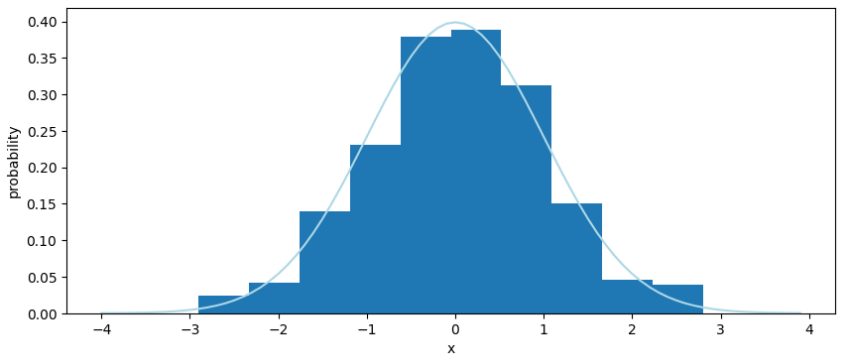
torch.randn_like でサンプリングされる値と、スクラッチ実装の正規分布との間に整合性があることが確認できた。
4. 多次元正規分布からデータをサンプリングする (未対応)
未対応
5. 対数確率密度 (log_probs / log_pis) の計算 (1次元正規分布から)
対数確率密度の計算式は、以下の記事に詳細に記載されている。
この計算は、強化学習エージェントの方策に対して、ある行動の確率密度を求める際に利用されています。
「(1) 行動のサンプリングを単純に正規分布から行っている場合」には上記記事の計算を踏襲できるのですが、
「(2) 正規分布からサンプリングした値に活性化関数 (tanh など) を適用している場合」には、この計算に補正が必要になります。こちらのパターンについては、「5-2.」で確認します。
5-1. 純粋に正規分布から行動をサンプリング
5-1-1. 数式
- $\pi(a|s) \sim \mathcal{N} (\mu, \sigma)$ のとき
- $p(a) = \frac{1}{\sqrt{2 \pi \sigma^2}} e^{-\frac{(a-\mu)^2}{2 \sigma^2}}$
この時は、対数確率密度は以下のように式展開ができる。
\begin{align}
\log \pi(a|s) &= \log p(a) \\
&= \log \left( \frac{1}{\sqrt{2 \pi \sigma^2}} e^{-\frac{(a-\mu)^2}{2 \sigma^2}} \right) \\
&= \log 1 - \log \sqrt{2 \pi \sigma^2} -\frac{(a-\mu)^2}{2 \sigma^2} \\
&= 0 - \frac{1}{2} \log 2\pi - \sigma -\frac{(a-\mu)^2}{2 \sigma^2} \\
&= -\frac{1}{2} \log 2\pi - \sigma -\frac{(a-\mu)^2}{2 \sigma^2}
\end{align}
5-1-2. 実装
mean = 4
std = 0.8
norm_dist = Normal(mean, std)

# 正規分布から行動をサンプリング
actions = norm_dist.sample(torch.Size([100]))
actions.shape

# ---- 出力結果 ----
torch.Size([100])
以下のように、 Normal のインスタンスの log_prob メソッドを用いると、対数確率密度を取得できる。
# 対数確率密度を計算
log_probs = norm_dist.log_prob(actions)
正しく取得できているか確認するために、以下のコードで描画する。
# 対数確率密度を描画して比較できるようにするため、確率密度に変換
probs = log_probs.exp()

# 比較対象として、行動のサンプルを大量に取得 (histgram にする)
sampled_actions = norm_dist.sample(torch.Size([5000]))


# 描画処理
fig, ax = plt.subplots(1, 1, figsize=(10, 4))

# pytorch の Normal から大量サンプリングした行動をヒストグラムとして描画
ax.hist(sampled_actions, density=True, label="sampled histgram from Normal");

# log_prob 経由で取得した、各行動の確率密度を描画
plt.scatter(actions, probs, color='red', label='density of probability of each action')

plt.xlabel("x (value of action)")
plt.ylabel("probability")
plt.legend()
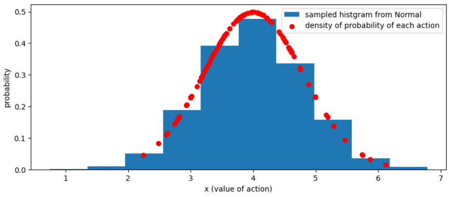
よさげ。
赤い点は、log_prob メソッド経由で取得した対数確率密度から計算された、各行動の生起確率であり、これらの点が、大量にサンプリングして作った histgram (青い棒グラフ) と一致している。
5-2. 正規分布からサンプリングした値を tanh に通してエージェントの行動とする
ここからが本題。
5-2-1. 数式
これは、以下のような場合を指している。
- $x \sim \mathcal{N} (\mu, \sigma)$
- $p(x) = \frac{1}{\sqrt{2 \pi \sigma^2}} e^{-\frac{(x-\mu)^2}{2 \sigma^2}}$
- $\pi(a|s) = \tanh(x)$
この場合は、対数確率密度は以下のように計算する。
\begin{align}
\log \pi(a|s) &= \log p(x) - \sum^D_{i=1} \log(1-\tanh^2(x_i)) \\
&= -\frac{1}{2} \log 2\pi - \sigma -\frac{(x-\mu)^2}{2 \sigma^2} - \sum^D_{i=1} \log(1-\tanh^2(x_i))
\end{align}
※この計算式の展開についての説明は、関連記事に載せてある「Soft Actor-Critic: Off-Policy Maximum Entropy Deep Reinforcement Learning with a Stochastic Actor」の論文を参照されたい。
5-2-2. 実装
mean = 5
std = 0.2
norm_dist = Normal(mean, std)

# 正規分布から x をサンプリング
x = norm_dist.sample(torch.Size([100]))

# tanh を使って行動へと変換
actions_tanh = torch.tanh(x)
actions_tanh.shape

# ---- 出力結果 ----
torch.Size([100])
以下のように、 Normal のインスタンスの log_prob メソッドを用いて、対数確率密度を取得する点は同じだが、途中から処理が追加されている。
# 対数確率密度を計算
log_prob_raw = norm_dist.log_prob(x)

# サンプリング後の値 x を tanh に通していることを考慮した補正項
correction = torch.log(1 - actions_tanh.pow(2) + 1e-6)

log_prob_corrected = log_prob_raw - correction
# 描画準備
# 比較できるように、対数を外す
prob_corrected = log_prob_corrected.exp()

# 比較対象として、大量の行動をサンプリング
sampled_actions = norm_dist.sample(torch.Size([5000]))
sampled_actions_tanh = torch.tanh(sampled_actions)

# 描画
fig, ax = plt.subplots(1, 1, figsize=(10, 4))

# pytorch の Normal から大量サンプリングした行動をヒストグラムとして描画
ax.hist(sampled_actions_tanh, density=True, label="sampled histgram from Normal");

# log_prob 経由で取得した、各行動の確率密度を描画
plt.scatter(actions_tanh, prob_corrected, color='red', label='density of probability of each action')

plt.xlabel("tanh(x) (value of action)")
plt.ylabel("probability")
plt.legend()
結果はこちら。
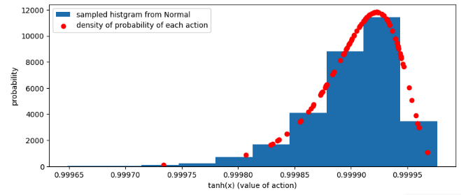
tanh を通した行動 (actions_tanh) の確率密度も、ヒストグラムの傾向に沿う値になっており、正しく計算できているようだ。
6. 対数確率密度 (log_probs / log_pis) の計算 (多次元正規分布から)
6-1. 純粋に正規分布から行動をサンプリング
多次元正規分布からサンプリングした値を、単純にエージェントの行動とする場合の確率密度の計算を実装する。
6-1-1. 数式
以下のように各変数を定義すると、
- $\mathbf{a} \in \mathbb{R}^d\ は d$ 次元の行動ベクトル
- $\boldsymbol{\mu} \in \mathbb{R}^d$ は平均ベクトル
- $\Sigma \in \mathbb{R}^{d \times d}$ は共分散行列
- $|\Sigma|$ は共分散行列の行列式
- $\Sigma^{-1}$ は共分散行列の逆行列
- $d$ は行動 (action) の次元数
\begin{align}
\pi(\mathbf{a}|\mathbf{s}) &\sim \mathcal{N} (\boldsymbol{\mu}, \Sigma) \\
p(\mathbf{a}) &= \frac{1}{(2\pi)^{\frac{d}{2}} |\Sigma|^{\frac{1}{2}}} \exp \left( -\frac{1}{2} (\mathbf{a} - \boldsymbol{\mu})^T \Sigma^{-1} (\mathbf{a} - \boldsymbol{\mu}) \right) \\
\\
\log p(\mathbf{a}) &= \log \left( \frac{1}{(2\pi)^{\frac{d}{2}} |\Sigma|^{\frac{1}{2}}} \right) + \log \exp \left( -\frac{1}{2} (\mathbf{a} - \boldsymbol{\mu})^T \Sigma^{-1} (\mathbf{a} - \boldsymbol{\mu}) \right) \\
&= -\frac{d}{2} \log (2\pi) - \frac{1}{2} \log |\Sigma| - \frac{1}{2} (\mathbf{a} - \boldsymbol{\mu})^T \Sigma^{-1} (\mathbf{a} - \boldsymbol{\mu})
\end{align}
6-1-2. 実装
mean = torch.Tensor([1, 3])
std = torch.Tensor([0.15, 0.055]) + 1e-8
norm_dist = Normal(mean, std)

# 正規分布から x をサンプリング
actions = norm_dist.sample(torch.Size([800]))
actions.shape

# ---- 出力結果 ----
torch.Size([800, 2])
対数確率密度の計算は、 tanh を通さないので単純。
# 対数確率密度を計算
log_probs = norm_dist.log_prob(actions).sum(dim=-1, keepdim=True)
この結果が正しいかどうか、確認するために描画してみよう。
# **** 描画準備 ****
xs = actions[:, 0]
ys = actions[:, 1]
# 比較できるように、対数を外す
zs = log_probs.exp()
print(xs.shape, ys.shape, zs.shape)
# 比較対象として、大量の行動をサンプリング
sampled_actions = norm_dist.sample(torch.Size([5000]))
# **** 描画 ****
fig = plt.figure()
ax = fig.add_subplot(projection='3d')
ax.scatter(xs, ys, zs.flatten(), marker='^', alpha=0.4, label="prob density")
# plot_3d_hist(sampled_actions[:, 0], sampled_actions[:, 1], ax=ax, density=True)
plt.legend()
plt.show()
# ---- 出力 ----
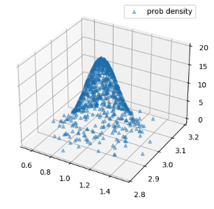
torch.Size([800]) torch.Size([800]) torch.Size([800, 1])
まず、計算した確率密度だけを描画した結果です。
大量にサンプリングした行動のヒストグラムを表示する場合は、以下のメソッドも使います。
描画に利用した関数
def plot_3d_hist(x, y, ax = None, bin_size: int = 15, density = False) -> None:
    """
    2次元の分布データから3次元ヒストグラムを描画
    https://phst.hateblo.jp/entry/2023/02/24/080000

    Parameters
    ------
    x: 1次元配列
    y: 1次元配列
    """
    # 描画データの準備
    _xrange = [min(x),max(x)]
    _yrange = [min(y),max(y)]
    bins = [bin_size, bin_size]
    N: int = bins[0] * bins[1]
    wbins = [(_xrange[1] - _xrange[0]) / bins[0], (_yrange[1] - _yrange[0]) / bins[1]]

    hist, edgesx, edgesy = np.histogram2d(x, y, bins=bins, range=[_xrange, _yrange])
    hist = np.flipud(np.rot90(hist)) # histogram2d 出力の仕様由来のおまじない

    if density:
        bin_area = wbins[0] * wbins[1]  # 各ビンの面積
        hist /= (hist.sum() * bin_area)  # ビンの面積を考慮して正規化

    xpos, ypos = np.meshgrid(edgesx[:-1], edgesy[:-1])
    xpos = xpos.flatten()
    ypos = ypos.flatten()
    zpos = np.array([0] * N)

    dx = np.array([wbins[0]] * N)
    dy = np.array([wbins[1]] * N)
    dz = hist.flatten()


    if ax is None:
        fig = plt.figure(figsize=(6, 6))
        ax = fig.add_subplot(projection='3d')

    # ax.bar3d(x=xpos[dz>0], y=ypos[dz>0], z=zpos[dz>0], dx=dx[dz>0], dy=dy[dz>0], dz=dz[dz>0], shade=True)
    ax.bar3d(x=xpos, y=ypos, z=zpos, dx=dx, dy=dy, dz=dz, shade=True, alpha=0.2, label="histgram for density func")
    ax.set_xlabel('X')
    ax.set_ylabel('Y')
    ax.set_zlabel('Z')
    ax.set_xlim(*_xrange)
    ax.set_ylim(*_yrange)


# 関数をテストするためのデータ
np.random.seed(3)
x0 = np.random.randn(10000)*0.5 + 4 #標準偏差0.5, 平均4の正規分布
y0 = np.random.randn(10000)*2   + 3 #標準偏差2.0, 平均3の正規分布
x1 = np.random.randn(1000)*0.5 + 0 #標準偏差0.5, 平均0の正規分布
y1 = np.random.randn(1000)*2   + 0 #標準偏差2.0, 平均0の正規分布

x=np.concatenate((x0,x1))
y=np.concatenate((y0,y1))

# 描画
plot_3d_hist(x,y)
plt.legend()
plt.show()

x.shape, y.shape
fig = plt.figure()
ax = fig.add_subplot(projection='3d')
ax.scatter(xs, ys, zs.flatten(), marker='^', alpha=0.4, label="prob density")

# plot_3d_hist の実装は、折りたたんである「描画に利用した関数」をご参照ください ^^
plot_3d_hist(sampled_actions[:, 0], sampled_actions[:, 1], ax=ax, density=True)
plt.legend()
plt.show()
以下のような結果になり、概ね正しそうです。

6-2. 正規分布からサンプリングした値を tanh に通してエージェントの行動としている場合
これが一番やりたかったことです!
行きますよ!!(๑•̀ㅂ•́)و
6-2-1. 数式
式変形はほぼ完全に ChatGPT に頼って導出しましたが、なんとか内容を理解できたので、私なりの補足も付け加えて記載します。
定義 (再掲)
- $\mathbf{a} \in \mathbb{R}^d\ は d$ 次元の行動ベクトル
- $\boldsymbol{\mu} \in \mathbb{R}^d$ は平均ベクトル
- $\Sigma \in \mathbb{R}^{d \times d}$ は共分散行列
- $|\Sigma|$ は共分散行列の行列式
- $\Sigma^{-1}$ は共分散行列の逆行列
- $d$ は行動 (action) の次元数
ーーーーーーーー 計算方針 ーーーーーーーー
-
変換前の行動:
多次元正規分布 $\mathcal{N}(\boldsymbol{\mu}, \Sigma)$ からサンプルを取得:
$$
\mathbf{z} \sim \mathcal{N}(\boldsymbol{\mu}, \Sigma)
$$
-
変換後の行動:
$\mathbf{z}$ を $\tanh$ に通して action を取得:
$$
\mathbf{a} = \tanh(\mathbf{z})
$$
確率密度の算出のために、変数変換 を行って対数確率密度を求めます2。 ヤコビアン行列の行列式の絶対値 を計算しなければなりません。
$$
p(\mathbf{a}) = p(\mathbf{z}) \left| \det \frac{d\mathbf{z}}{d\mathbf{a}} \right|
$$
これの対数を取ると、
$$
\log p(\mathbf{a}) = \log p(\mathbf{z}) + \log \left| \det \frac{d\mathbf{z}}{d\mathbf{a}} \right|
$$
ーーーーーーーー ヤコビアンの計算 ーーーーーーーー
$\mathbf{a} = \tanh(\mathbf{z})$ なので、各成分について導関数を求めると
$$
\frac{da_i}{dz_i} = 1 - \tanh^2(z_i)
$$
よって、対角行列としてヤコビアン行列は
$$
J = \text{diag} (1 - \tanh^2(z_1), 1 - \tanh^2(z_2), \dots, 1 - \tanh^2(z_d))
$$
その行列式は、
$$
\left| \det J \right| = \prod_{i=1}^{d} (1 - \tanh^2(z_i))
$$
対数を取ると、
$$
\log \left| \det J \right| = \sum_{i=1}^{d} \log (1 - \tanh^2(z_i))
$$
ーーーーーーーー 最終的な式 ーーーーーーーー
$$
\log p(\mathbf{a}) = \log p(\mathbf{z}) + \sum_{i=1}^{d} \log (1 - \tanh^2(z_i))
$$
ここで、
$$
\log p(\mathbf{z}) = -\frac{d}{2} \log (2\pi) - \frac{1}{2} \log |\Sigma| - \frac{1}{2} (\mathbf{z} - \boldsymbol{\mu})^T \Sigma^{-1} (\mathbf{z} - \boldsymbol{\mu})
$$
これを代入して、
$$
\log p(\mathbf{a}) = -\frac{d}{2} \log (2\pi) - \frac{1}{2} \log |\Sigma| - \frac{1}{2} (\mathbf{z} - \boldsymbol{\mu})^T \Sigma^{-1} (\mathbf{z} - \boldsymbol{\mu}) + \sum_{i=1}^{d} \log (1 - \tanh^2(z_i))
$$
数式の確認、お疲れさまでした!(o*。_。)o
実は、最後の項しか実装には必要ないんですけどね!!!理論的にどういう仕組みなのか気になったので調べてしまいました。
6-2-2. 実装
mean = torch.Tensor([1, 3])
std = torch.Tensor([0.15, 0.055]) + 1e-8
log_stds = torch.log(std)

# 正規分布から x をサンプリング
norm_dist = Normal(mean, std)
z_raw_actions = norm_dist.rsample(torch.Size([500]))

# tanh を使って行動へと変換
actions = torch.tanh(z_raw_actions)
actions.shape  # , actions

# ---- 出力結果 ----
torch.Size([200, 2])
# 対数確率密度を計算
log_prob_z = norm_dist.log_prob(z_raw_actions).sum(dim=-1, keepdim=True)

# サンプリング後の値 z を tanh に通していることを考慮した補正項
correction = torch.log(1 - actions.pow(2) + 1e-8).sum(dim=-1, keepdim=True)

log_prob_a = log_prob_z - correction
# 描画準備
# 比較できるように、対数を外す
prob_corrected = log_prob_a.exp()
# print(log_prob_a, correction,  prob_corrected)
# prob_corrected.shape

# 比較対象として、大量の行動をサンプリング
sampled_actions = norm_dist.rsample(torch.Size([5000]))
sampled_actions_tanh = torch.tanh(sampled_actions)
まずは、サンプリングした行動の対数確率密度だけを描画。
# 描画
xs = actions[:, 0]
ys = actions[:, 1]
zs = prob_corrected

# https://matplotlib.org/stable/gallery/mplot3d/scatter3d.html
fig = plt.figure()
ax = fig.add_subplot(projection='3d')
ax.scatter(xs, ys, zs.flatten(), marker='^', alpha=0.2)
plt.show()

次に、行動の分布のヒストグラムを描画してみる。
plot_3d_hist(sampled_actions_tanh[:, 0].numpy(), sampled_actions_tanh[:, 1].numpy(), density=True)
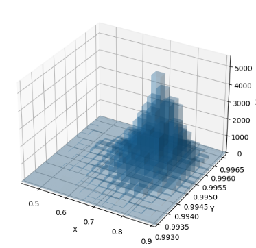
ほとんど同じ形状!( *˙︶˙*)وグッ!
では重ねて描画してみよう。
# 描画
xs = actions[:, 0]
ys = actions[:, 1]
zs = prob_corrected

print(xs.shape, ys.shape, zs.shape)

# https://matplotlib.org/stable/gallery/mplot3d/scatter3d.html
fig = plt.figure()
ax = fig.add_subplot(projection='3d')
ax.scatter(xs, ys, zs.flatten(), marker='^', alpha=0.2)

plot_3d_hist(sampled_actions_tanh[:, 0].numpy(), sampled_actions_tanh[:, 1].numpy(), ax=ax, density=True)

plt.show()

ほとんど完全に一致している!
正しく確率密度関数の計算が行えていることが、これで確認できた。
6-3. 正規分布からサンプリングした値を tanh 関数に通し、その上で scaling を行って Action とする場合
6-3-1. 数式
6-2-1. からわずかな変化があります。
定義 (再掲)
- $\mathbf{a} \in \mathbb{R}^d\ は d$ 次元の行動ベクトル
- $\boldsymbol{\mu} \in \mathbb{R}^d$ は平均ベクトル
- $\Sigma \in \mathbb{R}^{d \times d}$ は共分散行列
- $|\Sigma|$ は共分散行列の行列式
- $\Sigma^{-1}$ は共分散行列の逆行列
- $d$ は行動 (action) の次元数
- $scale$ は tanh の出力にかけて値の範囲をコントロールするための定数
- $bias$ は tanh の出力を scale した後に加算される定数
ーーーーーーーー 計算方針 ーーーーーーーー
-
変換前の行動:
多次元正規分布 $\mathcal{N}(\boldsymbol{\mu}, \Sigma)$ からサンプルを取得:
$$
\mathbf{z} \sim \mathcal{N}(\boldsymbol{\mu}, \Sigma)
$$
-
tanh 変換後の行動:
$\mathbf{z}$ を $\tanh$ に通して action を取得:
$$
\mathbf{a} = \tanh(\mathbf{z})
$$
- scaling 後の行動:
$$
\mathbf{a_scaled} = \tanh(\mathbf{z}) * scale + bias
$$
ーーーーーーーー 最終的な式 ーーーーーーーー
導出過程はわかりませんでしたが。。。実装と動作確認から数式の正しさを確認しました。
$$
\log p(\mathbf{a}) = \log p(\mathbf{z}) + \sum_{i=1}^{d} \log (1 - \tanh^2(z_i)) + \log(scaling)
$$
ここで、
$$
\log p(\mathbf{z}) = -\frac{d}{2} \log (2\pi) - \frac{1}{2} \log |\Sigma| - \frac{1}{2} (\mathbf{z} - \boldsymbol{\mu})^T \Sigma^{-1} (\mathbf{z} - \boldsymbol{\mu})
$$
これを代入して、
$$
\log p(\mathbf{a}) = -\frac{d}{2} \log (2\pi) - \frac{1}{2} \log |\Sigma| - \frac{1}{2} (\mathbf{z} - \boldsymbol{\mu})^T \Sigma^{-1} (\mathbf{z} - \boldsymbol{\mu}) + \sum_{i=1}^{d} \log (1 - \tanh^2(z_i)) + \log(scaling)
$$
6-3-2. 実装
実装もごくわずかにしか変わりません。
6-2-2. との差分がある箇所のみ 緑 にしておきます。正式な diff の使い方とは違いますが。。。。
+ # scaling パラメータ
+ action_bias = 3.0
+ action_scale = 10.0

mean = torch.Tensor([1, 3])
std = torch.Tensor([0.15, 0.055]) + 1e-8
log_stds = torch.log(std)

# 正規分布から x をサンプリング
norm_dist = Normal(mean, std)
z_raw_actions = norm_dist.rsample(torch.Size([500]))

# tanh を使って行動へと変換
actions = torch.tanh(z_raw_actions)

+ # 出力に対する scaling
+ scaled_actions = actions * action_scale + action_bias
# 対数確率密度を計算
log_prob_z = norm_dist.log_prob(z_raw_actions)

# サンプリング後の値 z を tanh に通していることを考慮した補正項
correction = torch.log(1 - actions.pow(2) + 1e-8)  # tanh'(z) = 1 - tanh^2(z)
+ correction += np.log(action_scale)
log_prob_a = torch.sum(log_prob_z - correction, dim=-1, keepdim=True)

# 描画準備
# 比較できるように、対数を外す
prob_corrected = log_prob_a.exp()
prob_corrected.shape
# 比較対象として、大量の行動をサンプリング
sampled_actions_raw = norm_dist.rsample(torch.Size([5000]))
sampled_actions_tanh = torch.tanh(sampled_actions_raw)

+ # 同様に scaling
+ sampled_actions_scaled = sampled_actions_tanh * action_scale + action_bias
+ sampled_actions_scaled.shape
- まず、計算した確率密度を描画します
# 描画
+ xs = scaled_actions[:, 0]
+ ys = scaled_actions[:, 1]
zs = prob_corrected

print(xs.shape, ys.shape, zs.shape)

# https://matplotlib.org/stable/gallery/mplot3d/scatter3d.html
fig = plt.figure()
ax = fig.add_subplot(projection='3d')
ax.scatter(xs, ys, zs.flatten(), marker='^', alpha=0.2)
plt.show()

- 次にサンプリングされた行動のヒストグラムを表示
+ plot_3d_hist(sampled_actions_scaled[:, 0].numpy(), sampled_actions_scaled[:, 1].numpy(), density=True)
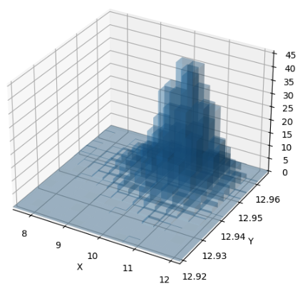
形状はほぼ一緒ですね!
重ねてグラフに出力してみましょう。
# 描画
+ xs = scaled_actions[:, 0]
+ ys = scaled_actions[:, 1]
zs = prob_corrected

print(xs.shape, ys.shape, zs.shape)

# https://matplotlib.org/stable/gallery/mplot3d/scatter3d.html
fig = plt.figure()
ax = fig.add_subplot(projection='3d')
ax.scatter(xs, ys, zs.flatten(), marker='^', alpha=0.2)

+ plot_3d_hist(sampled_actions_scaled[:, 0].numpy(), sampled_actions_scaled[:, 1].numpy(), ax=ax, density=True)

plt.show()

座標と高さがほぼ一致していますね!
これで計算が正しそうなことが確認できました( *¯ ꒳¯*)✨
関連記事
1. tanh / arctanh の計算式
2. pytorch 公式ドキュメント: torch.distributions.Normal について
- Probability distributions - torch.distributions / Normal
3. pytorch の distributions.Normal クラスにおける log_prob メソッドの実装
4. 【Soft Actor-Critic】Action の値を tanh に通す場合の確率密度についての理論的説明
- Soft Actor-Critic: Off-Policy Maximum Entropy Deep Reinforcement Learning with a Stochastic Actor
- Appendix - C. Enforcing Action Bounds を参照
5. matplotlib で3次元空間上に scatter を描画
6. 3次元のヒストグラムを描画する
- 2次元の分布データから3次元ヒストグラムを描画する方法は、以下の記事のコードをほぼ流用しました
7. 確率密度関数の変数変換の公式
-
GitHub: 対数確率密度の計算を実装した ipynb ファイルのアップロード先リンク - https://github.com/siruku6/thesis-trial/blob/master/reinforcement_learning/250523_torch_trial_for_advantage_log_prob.ipynb ↩
-
確率密度関数の変数変換の仕方については、次の記事が参考になる - (https://ushitora.net/archives/954) 関連記事「7.」に掲載している記事と同一の記事である ↩