量子ビットをイメージでつかむ（振幅増幅編）

　本記事は量子もつれ編の続きとなります。引き続きこちらを教科書としています。Jupyter notebookを https://github.com/sin-gee/ImageOfQuantumBit/ImageOfGrover.ipynb に置いておきますのでよろしければ試してみてください。

---

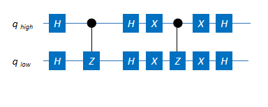
　今回、目指す量子回路は次のとおりです。

この回路は、大きく次のように分割できると思います。

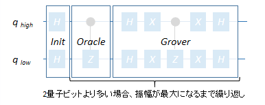
各ブロックに分けて見ていきます。

---

最初の$H \otimes H$は初期化で、$\lvert s\rangle=\frac{1}{2}(\lvert00\rangle+\lvert01\rangle+\lvert10\rangle+\lvert01\rangle+\lvert11\rangle)$の状態を作っています。ちなみに$n$ビットの場合は、$\lvert s\rangle=H^{\otimes n}\lvert0\rangle^{\otimes n}=\frac{1}{\sqrt{2^n}}\sum_{x=0}^{2^n-1}\lvert x\rangle$となります。

---

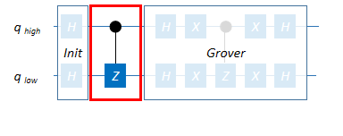
　次の$Oracle$（CZ）は、狙いの$\lvert11\rangle$の正負の符号を反転させます。CZを使ったのは、あくまで$\lvert11\rangle$の振幅を増幅させるためです。他の振幅を増幅させる場合はどう回路を組めば良いか考えどころですが、振幅増幅のメカニズムを考える上では本質でないと思いますので、Jupyter notebook上では次の関数で代用してます。

#汎用Zゲート 
def z_gate(q00,q01,q10,q11,target):
    if target=='00':
      q00_ = -q00
      q01_ = q01
      q10_ = q10
      q11_ = q11
    elif target=='01':
      q00_ = q00
      q01_ = -q01
      q10_ = q10
      q11_ = q11
    elif target=='10':
      q00_ = q00
      q01_ = q01
      q10_ = -q10
      q11_ = q11 
    elif target=='11':
      q00_ = q00
      q01_ = q01
      q10_ = q10
      q11_ = -q11
    else:
      q00_ = q00
      q01_ = q01
      q10_ = q10
      q11_ = q11
      print('CZ gate not changed')

式にすると、
$U_f\lvert s\rangle = \frac{1}{\sqrt{2^n}}\sum_{x=0,x\neq w}^{2^n-1}\lvert x\rangle-\frac{1}{\sqrt{2^n}}\lvert w\rangle = \lvert s\rangle-\frac{2}{\sqrt{2^n}}\lvert w\rangle
$
と、ちょっとげっそりですが、（３次元の）絵にすると一目瞭然です。

つまり$\lvert s\rangle$を$\lvert 11\rangle$以外のすべての基底が作る（超）平面の反対側に持ってこようとしている訳です。

---

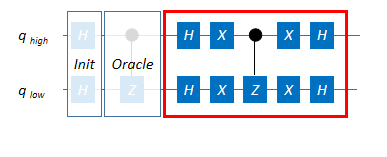
　$Oracle$に続く$Grover$はちょっと複雑な感じです。ここでもCZが使われていますが、これは$Oracle$とは違い、増幅する対象には依存しません。ちなみに3量子ビットの場合はCCZで、$\lvert111\rangle$がターゲットビットになります。
　教科書によると、式としては $U_s=2\lvert s\rangle\langle s\rvert - I$だそうです。これは、どういうものか、次のコードで確認してみます。

import numpy as np
import numpy.linalg as LA

dims = 2**2 # 2量子ビットのため次元数は2^2となる
x = (1/dims**0.5)
one = np.ones((dims,1))
sKet = x*one             # |s>を求める
sBra = np.transpose(sKet)# <s|を求める
print('|s>')
print(sKet)
print('<s|')
print(sBra)
I = np.eye(dims) #単位行列
print('I')
print(I)
print('G')
G =  2*np.dot(sKet,sBra) - I # 2|s><s| - I
print(G)
# 固有値、逆行列を計算してユニタリー行列であることを確認する
l, p = LA.eig(G)
print("固有値")
print(l)  # 固有値
print("逆行列 ")
print(np.linalg.inv(G))

　固有値の絶対値はすべて１、逆行列（の複素共役）と自身が一致することからユニタリー行列です。では、この行列（ゲート）が何をするのか次のコードで確認してみます。

def vector_to_vector_rotation_angle(v1, v2): #２ベクトルの角度をπ単位で算出
    return  np.arccos(np.inner(v1,v2)/(np.dot(np.linalg.norm(v1),np.linalg.norm(v2))))

q00 = np.array([[1],[0],[0],[0]]) # Try any Vector
t00 = np.dot(G,q00)
print(t00)

print('変換前と変換後に点対称にしたベクトルの間の角度は',round(vector_to_vector_rotation_angle(q00.reshape(-1),t00.reshape(-1))/np.pi,3),'pi')
print('変換前のベクトルと|s>との間の角度は',round(vector_to_vector_rotation_angle(q00.reshape(-1),sKet.reshape(-1))/np.pi,3),'pi')
print('変換後に点対称にしたベクトルと|s>との間の角度は',round(vector_to_vector_rotation_angle(sKet.reshape(-1),t00.reshape(-1))/np.pi,3),'pi')

つまり、こういうことです。

　このゲートは、任意のベクトルを$\lvert s\rangle$の反対側に持っていく操作を行っています。これが増幅振幅の正体という訳です。

　では、では先ほどの量子回路は、この$2\lvert s\rangle\langle s\rvert - I$を実現しているのでしょうか？次のコードで確かめてみます。

HxH = 0.5*np.array([[ 1, 1, 1, 1],
                    [ 1,-1, 1,-1],
                    [ 1, 1,-1,-1],
                    [ 1,-1,-1, 1]])
XxX =     np.array([[ 0, 0, 0, 1],
                    [ 0, 0, 1, 0],
                    [ 0, 1, 0, 0],
                    [ 1, 0, 0, 0]])
CZ  =     np.array([[ 1, 0, 0, 0],
                    [ 0, 1, 0, 0],
                    [ 0, 0, 1, 0],
                    [ 0, 0, 0,-1]])

print('Grover回路の各段階の様子')

print('1回目のアダマール後')
G_1 = np.dot(HxH,I)
print(G_1)

print('1回目のXゲート後')
G_2 = np.dot(XxX,G_1)
print(G_2)

print('CZゲート後')
G_3 = np.dot(CZ,G_2)
print(G_3)

print('2回目のXゲート後')
G_4 = np.dot(XxX,G_3)
print(G_4)

print('2回目のHゲート後')
G_5 = np.dot(HxH,G_4)
print(G_5)

　どうでしょう？同じにはなりませんね。ちょうどマイナス１を掛けたものになるハズです。これで問題ないのか？問題ないです。マイナス１はグローバル位相としてキャンセルされます。位相は反対（マイナス）側でも振幅には問題ない、という訳です。

---

以下、説明の中の図を作成したコード

import numpy as np
import math
import matplotlib.pyplot as plt
from mpl_toolkits.mplot3d import Axes3D

d = 3 # 次元数　np.sqrt(2**n) nは量子ビット数 今回は3次元で描画

# 各次元のベクトルを指定
u, v, w = 1/(d**0.5), 1/(d**0.5), 1/(d**0.5)

# 矢印プロットを作成
fig = plt.figure(figsize=(8, 8)) # 図の設定
ax = fig.add_subplot(projection='3d') # 3Dプロットの設定
ax.quiver(0, 0, 0, u, v, w, arrow_length_ratio=0.2,color='blue') # |s>
ax.quiver(0, 0, 0, u, 0, 0, arrow_length_ratio=0.1, color='black') # |00>
ax.quiver(0, 0, 0, 0, v, 0, arrow_length_ratio=0.1, color='black') # |01>
ax.quiver(0, 0, 0, 0, 0, w, arrow_length_ratio=0.1, color='green') # |11>
ax.quiver(u, v, w, 0, 0, -w, arrow_length_ratio=0.1, lw=0.5, color='green') # |w>
ax.quiver(u, v, 0, 0, 0, -w, arrow_length_ratio=0.1, lw=0.5,color='green') # |w>
ax.quiver(0, 0, 0, u, v, -w, arrow_length_ratio=0.1,linestyle='--',color='blue') # |s>-2|w>


plt.plot([-1.0,1.0], [0, 0], [0, 0],color='gray',linestyle=':') 
plt.plot([0,0], [-1.0, 1.0], [0, 0],color='gray',linestyle=':') 
plt.plot([0,0], [0, 0], [-1.0, 1.0],color='gray',linestyle=':') 


theta_1_0 = np.linspace(0, 2*np.pi, 100) 
theta_2_0 = np.linspace(0, 2*np.pi, 100) 
theta_1, theta_2 = np.meshgrid(theta_1_0, theta_2_0) 
cx = np.cos(theta_2)*np.sin(theta_1) 
cy = np.sin(theta_2)*np.sin(theta_1)  
cz = np.cos(theta_1) 
ax.plot_surface(cx,cy,cz, alpha=0.05) # 球表示

theta = np.linspace(np.pi-math.acos(1/d**0.5), math.acos(1/d**0.5), 20) 
x_c = np.cos(np.pi/4)*np.sin(theta)*0.25
y_c = np.sin(np.pi/4)*np.sin(theta)*0.25
z_c = np.cos(theta)*0.25
ax.plot(x_c, y_c, z_c, color="r")


ax.text(1.1, 0, 0, s=r'$|00\rangle$', fontsize=10)
ax.text(0.1, 1.1, 0, s=r'$|01\rangle$', fontsize=10)
ax.text(0.1, 0,1.1, s=r'$|11\rangle$', fontsize=10)

ax.text(u*1.3, v*1.1, w*1.1, s=r'$|s\rangle$',color='blue', fontsize=12)

ax.text(-0.05,  0, 0.25, s=r'$1/\sqrt{2^n}|w\rangle$',color='green',fontsize=12)
ax.text(u*2.3,  v*1.6, 0.4, s=r'$-1/\sqrt{2^n}|w\rangle$',color='green',fontsize=12)
ax.text(u*2.3,  v*1.6, -0.1, s=r'$-1/\sqrt{2^n}|w\rangle$',color='green',fontsize=12)

ax.text(0.35, 0.3, -0.05, s=r'$\theta$',color='red',fontsize=12)


ax.set_xlim(-1.1, 1.1) # x軸の表示範囲
ax.set_ylim(-1.1, 1.1) # y軸の表示範囲
ax.set_zlim(-1.1, 1.1) # z軸の表示範囲

ax.set_box_aspect((1,1,1))
ax.set_title('Oracle', fontsize=20,x=0.5,y=0.9) # タイトル
plt.axis('off')

ax.view_init(elev=10, azim=60) #視点の設定

import numpy as np
import math
import matplotlib.pyplot as plt
from mpl_toolkits.mplot3d import Axes3D

d = 3 # 次元数　np.sqrt(2**n) nは量子ビット数 今回は3次元で描画

# 各次元の変化量を指定
u, v, w = 1/(d**0.5), 1/(d**0.5), 1/(d**0.5)

# 矢印プロットを作成
fig = plt.figure(figsize=(8, 8)) # 図の設定
ax = fig.add_subplot(projection='3d') # 3Dプロットの設定
ax.quiver(0, 0, 0, u, v, w, arrow_length_ratio=0.1,color='gray') # |s>
ax.quiver(0, 0, 0, u, 0, 0, arrow_length_ratio=0.1, color='black') # |00>
ax.quiver(0, 0, 0, 0, v, 0, arrow_length_ratio=0.1, color='black') # |01>
ax.quiver(0, 0, 0, 0, 0, w, arrow_length_ratio=0.1, color='black') # |11>
ax.quiver(0, 0, 0, u, v, -w, arrow_length_ratio=0.1,linestyle='--',color='blue') # |s> -2|w>
t = math.acos(1/d**0.5)-2*math.asin(1/d**0.5)
ax.quiver(0, 0, 0, np.cos(np.pi/4)*np.sin(t), np.sin(np.pi/4)*np.sin(t),np.cos(t) , arrow_length_ratio=0.2,color='blue') #振幅増幅後


plt.plot([-1.1,1.1], [0, 0], [0, 0],color='gray',linestyle=':') 
plt.plot([0,0], [-1.1, 1.1], [0, 0],color='gray',linestyle=':') 
plt.plot([0,0], [0, 0], [-1.1, 1.1],color='gray',linestyle=':') 


theta_1_0 = np.linspace(0, 2*np.pi, 100) 
theta_2_0 = np.linspace(0, 2*np.pi, 100) 
theta_1, theta_2 = np.meshgrid(theta_1_0, theta_2_0) 
cx = np.cos(theta_2)*np.sin(theta_1) 
cy = np.sin(theta_2)*np.sin(theta_1)  
cz = np.cos(theta_1) 
ax.plot_surface(cx,cy,cz, alpha=0.05) # 球表示


theta = np.linspace( math.acos(1/d**0.5),t, 20) 
x_c = np.cos(np.pi/4)*np.sin(theta)*0.25
y_c = np.sin(np.pi/4)*np.sin(theta)*0.25 
z_c = np.cos(theta)*0.25
ax.plot(x_c, y_c, z_c, color="r")

theta = np.linspace(np.pi-math.acos(1/d**0.5) ,math.acos(1/d**0.5),20) 
x_c = np.cos(np.pi/4)*np.sin(theta)*0.20
y_c = np.sin(np.pi/4)*np.sin(theta)*0.20
z_c = np.cos(theta)*0.20
ax.plot(x_c, y_c, z_c, color="r")

theta = np.linspace(np.pi-math.acos(1/d**0.5),t, 20) 
x_c = np.cos(np.pi/4)*np.sin(theta)*0.4
y_c = np.sin(np.pi/4)*np.sin(theta)*0.4
z_c = np.cos(theta)*0.4
ax.plot(x_c, y_c, z_c, color="r")


ax.text(0.1, 0, 1.1, s=r'$|11\rangle$', fontsize=10)
ax.text(1.2, 0, 0, s=r'$|00\rangle$', fontsize=10)
ax.text(0.1, 1.2, 0, s=r'$|01\rangle$', fontsize=10)
ax.text(u*1.3, v*1.1, w*1.1, s=r'$|s\rangle$',color='gray', fontsize=12)
ax.text(0.1, 0, 0.25, s=r'$\theta$',color='red',fontsize=12)
ax.text(0.23, 0.15,-0.05, s=r'$\theta$',color='red',fontsize=12)
ax.text(0.18, 0, 0.45, s=r'$2\theta$',color='red',fontsize=12)


ax.set_xlim(-1.1, 1.1) # x軸の表示範囲
ax.set_ylim(-1.1, 1.1) # y軸の表示範囲
ax.set_zlim(-1.1, 1.1) # z軸の表示範囲

ax.set_box_aspect((1,1,1))
ax.set_title('Grover', fontsize=20,x=0.5,y=0.9) # タイトル
plt.axis('off')

ax.view_init(elev=10, azim=70) #視点の設定