今回はQuick, Draw! Doodle Recognition Challenge
/ How accurately can you identify a doodle?のKaggleコンテストで遊んでみます。
コンテスト概要
Quick, Drawという、落書きを書いてそれをAIが予測するwebアプリ?のデータセットに対する、クラスタリングのコンテストです。
そういえば、アプリ自体は会社でも昔話題になったような気もします。
コンテスト参加時の認証
今回から、初の賞金が絡むコンテストになるので、初回のみのSMS認証が必要になりました。
最初携帯にメールが届かず・・調べていたら、My SoftBankの「迷惑メール対策の詳細設定」というページのSMSタブに、「海外事業者からの電話番号メールをすべて拒否します。」という設定が・・詳細設定画面やらタブ切り替えで奥まったページにあり、気づきませんでした・・![]()
設定変更したら、無事メールが届き、コンテスト参加となりました。
データチェック
今回も、データセットの配置などが楽なように、Kaggle Kernelを利用していきます。
また、おそらくディープラーニングも使うことになりそうなので、GPUを有効にしておきます。
import numpy as np
import pandas as pd
import os
print(os.listdir("../input"))
['test_simplified.csv', 'sample_submission.csv', 'train_simplified', 'test_raw.csv']
なにやらsimplifiedとrawというものがあるらしい。
コンテストの説明を読むと、simplifiedは無駄なデータを省いたデータとのこと。どちらを使っても、もしくは両方使ってもOKらしいです。
とりあえずはsimlifiedの方で進めてみます。
simplified_file_name_list = os.listdir("../input/train_simplified/")
simplified_file_name_list
['sleeping bag.csv',
 'house plant.csv',
 'bathtub.csv',
 'key.csv',
 'triangle.csv',
 'grapes.csv',
 ...]
len(simplified_file_name_list)
340
ファイル多いな!
とりあえず部分的にファイルの内容を確認してみます。
simplified_file_path_list = []
for simplified_file_name in simplified_file_name_list:
    simplified_file_path_list.append(
        '../input/train_simplified/%s' % simplified_file_name)
df = pd.read_csv(simplified_file_path_list[0])
df.head(n=3)
| countrycode | drawing | key_id | recognized | timestamp | word | |
|---|---|---|---|---|---|---|
| 0 | US | [[[92, 91, 82, 69, 64, 56, 28, 15, 6, 0, 1, 18... | 4745881255411712 | True | 2017-03-10 13:46:31.635970 | sleeping bag |
| 1 | US | [[[52, 22, 12, 5, 1, 0, 5, 26, 149, 184, 230, ... | 4859794726846464 | False | 2017-03-04 17:08:46.745630 | sleeping bag |
| 2 | AU | [[[4, 3, 11, 22, 38, 63, 251, 255, 251, 252, 2... | 4573190200229888 | True | 2017-03-17 06:36:27.083520 | sleeping bag |
df.info()
<class 'pandas.core.frame.DataFrame'>
RangeIndex: 119691 entries, 0 to 119690
Data columns (total 6 columns):
countrycode    119687 non-null object
drawing        119691 non-null object
key_id         119691 non-null int64
recognized     119691 non-null bool
timestamp      119691 non-null object
word           119691 non-null object
dtypes: bool(1), int64(1), object(4)
memory usage: 4.7+ MB
countrycodeは欠損値がある模様。本当はすべてのCSVをチェックした方がいいのですが、仕事ではないのでスキップします。
drawingカラムの内容を少し詳しく見てみます。
df.loc[0, 'drawing']
'[[[92, 91, 82, 69, 64, 56, 28, 15, 6, 0, 1, 18, 27, 54, 69, 83, 92, 92], [143, 78, 60, 15, 6, 0, 1, 14, 29, 85, 224, 250, 253, 255, 246, 227, 184, 105]], [[59, 39, 13, 10, 38], [73, 80, 80, 74, 81]]]'
座標情報・・?でしょうか?少しデータ説明を詳しく読みます。
どうやらgithubに詳しい説明があるらしい。
https://github.com/googlecreativelab/quickdraw-dataset#the-raw-moderated-dataset
[
  [  // First stroke
    [x0, x1, x2, x3, ...],
    [y0, y1, y2, y3, ...],
    [t0, t1, t2, t3, ...]
  ],
  [  // Second stroke
    [x0, x1, x2, x3, ...],
    [y0, y1, y2, y3, ...],
    [t0, t1, t2, t3, ...]
  ],
  ... // Additional strokes
]
Where x and y are the pixel coordinates, and t is the time in milliseconds since the first point. x and y are real-valued while t is an integer. The raw drawings can have vastly different bounding boxes and number of points due to the different devices used for display and input.
なるほど。とりあえずはx座標をy座標の値だけ使っていきましょうか。(RNNとかも絡めるのなら時間情報も必要になってきそうではありますが・・)
We've simplified the vectors, removed the timing information, and positioned and scaled the data into a 256x256 region. The data is exported in ndjson format with the same metadata as the raw format. The simplification process was:
simplifiedの方は時間情報はなく、xとyの0~255までの値になっているそうなので、こちらを使っていきます。
一応、他のCSVも同じカラム構造になっていることを確認しておきます。
expected_columns_list = sorted(df.columns.tolist())
for simplified_file_path in simplified_file_path_list:
    df = pd.read_csv(simplified_file_path, nrows=10)
    columns_list = sorted(df.columns.tolist())
    assert columns_list == expected_columns_list
カラム構造の方はすべて一致しているようです。
test_simplified.csv側を見てみます。
test_simplified_df = pd.read_csv('../input/test_simplified.csv')
test_simplified_df.head(n=3)
| key_id | countrycode | drawing | |
|---|---|---|---|
| 0 | 9000003627287624 | DE | [[[17, 18, 20, 25, 137, 174, 242, 249, 251, 25... |
| 1 | 9000010688666847 | UA | [[[174, 145, 106, 38, 11, 4, 4, 15, 29, 78, 16... |
| 2 | 9000023642890129 | BG | [[[0, 12, 14, 17, 16, 24, 55, 57, 60, 79, 82, ... |
len(test_simplified_df)
112199
提出対象は約11万行。
どうするか考える。
データを見ていて、とりあえず、
- データが画像ではなく、座標の推移で表現されている。
- データ量はざっくり概算で、11万行×340クラス = 3740万くらいの落書きデータになり、大分多い
という点が気になります。
最初の方針として、以下のような形で進めたいと思います。
- 今回は、締め切りまでそれなりに期間があるため、最初から他人のカーネルは読み進めずに、自分で適当に進めてみてシンプルなもので一旦提出まで進める。(最下位の方でもとりあえず気にせず進める)
- 来週以降などに、他人のカーネルも読み進めて、参考にする。
- まず最初は、各クラスの画像を3000件までに制限し、且つそれらを座標ではなく画像に変換して扱えないか試してみる。(3000件でも、100万件程度になると思われるので、果たしてPILなどで捌けるのか否か・・)
- 画像サイズは、32px($\frac{1}{8}$)あたりまで縮小し、且つ白黒のMNIST的な画像にしておく。
- それらを、ニューラルネットワークでシンプルに推論してみる。(データ量的に増やしたときにいけるのかな・・カラーチャンネルないし、何とかなりそうな印象も・・)
- 提出は、各クラスを3つまで設定という記述があったので、確率で推論して上位3位までを使う。
画像変換の検証
1画像当たりの処理時間が長すぎるとしんどいことになるので、少し処理を検証してみます。
import json

from IPython.display import display
from PIL import Image, ImageDraw

df = pd.read_csv(simplified_file_path_list[3])
df.head(1)
| countrycode | drawing | key_id | recognized | timestamp | word | |
|---|---|---|---|---|---|---|
| 0 | US | [[[4, 0, 2], [202, 98, 24]], [[1, 12, 10, 25, ... | 5223042911305728 | True | 2017-03-18 02:52:34.909590 | key |
検証として、本当に処理が合っているか確認しやすいように、鍵(key)クラスを選択します。(最初、先頭の寝袋のクラスのままやっていたら、合っているのかよく分からなかった・・)
drawing_str_list = df['drawing'].tolist()
key_id_list = df['key_id'].tolist()


def display_32px_img(stroke_str):
    stroke_list = json.loads(stroke_str)
    target_img = Image.new(mode='1', size=(32, 32))
    target_draw = ImageDraw.Draw(im=target_img, mode='1')
    for unit_stroke_list in stroke_list:
        x_coord_list = unit_stroke_list[0]
        y_coord_list = unit_stroke_list[1]
        div_val = 8

        for i in range(len(x_coord_list)):
            if i == 0:
                continue
            x = int(x_coord_list[i] / div_val)
            y = int(y_coord_list[i] / div_val)
            pre_x = int(x_coord_list[i - 1] / div_val)
            pre_y = int(y_coord_list[i - 1] / div_val)
            target_draw.line(xy=(pre_x, pre_y, x, y), fill='#ffffff', width=2)
    display(target_img)
    target_img.close()
いくつか表示してみます。
for i in range(20):
    display_32px_img(stroke_str=drawing_str_list[i])
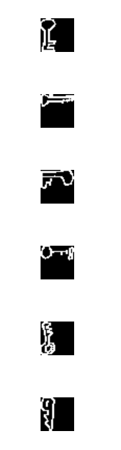
MNISTっぽい画像が作れました。また、形もなんとなく鍵っぽい画像で、処理は合っていそうです。
先ほどの関数を調整して、画像の表示ではなく配列を返却する関数にしてみます。
def get_32px_img_arr(stroke_str):
    stroke_list = json.loads(stroke_str)
    target_img = Image.new(mode='L', size=(32, 32))
    target_draw = ImageDraw.Draw(im=target_img, mode='L')
    for unit_stroke_list in stroke_list:
        x_coord_list = unit_stroke_list[0]
        y_coord_list = unit_stroke_list[1]
        div_val = 8

        for i in range(len(x_coord_list)):
            if i == 0:
                continue
            x = int(x_coord_list[i] / div_val)
            y = int(y_coord_list[i] / div_val)
            pre_x = int(x_coord_list[i - 1] / div_val)
            pre_y = int(y_coord_list[i - 1] / div_val)
            target_draw.line(xy=(pre_x, pre_y, x, y), fill='#ffffff', width=2)

    img_arr = np.asarray(target_img)
    return img_arr
なお、途中でデータを触っていて、2値画像よりもグレースケールの方が、PILとNumPy間のデータの変換がやりやすい(2値だと画像が崩れました・・特殊な指定が必要?)ので、mode='L'に変更してあります。
試しに、配列をPILに変換してみて、画像が崩れていないことを確認します。
img_arr = get_32px_img_arr(stroke_str=drawing_str_list[0])
img = Image.fromarray(img_arr)
img

大丈夫そうですね。
1枚当たりの時間を計ってみます。
%timeit get_32px_img_arr(stroke_str=drawing_str_list[0])
431 µs ± 11.8 µs per loop (mean ± std. dev. of 7 runs, 1000 loops each)
100万枚処理するとして、大体431 * 1000000 / 1000 / 1000 / 60 = 7.2分くらいです。遅くもないですが・・最初なのでさくっと変換が終わるようにしておいて、カーネルを再起動した後にも楽ができるように、少し調整しておきます。
また、学習面でも少し早くなるかな・・ということで、MNISTと合わせて28pxにしてさらに画像を小さくし、ujsonモジュールの方を使う形に調整しておきます。(とはいっても、変換のところはほとんどの処理時間がPILのline関数のところのようなので、ほとんど変わりません。)
import ujson

def get_28px_img_arr(stroke_str):
    stroke_list = ujson.loads(stroke_str)
    target_img = Image.new(mode='L', size=(28, 28))
    target_draw = ImageDraw.Draw(im=target_img, mode='L')
    for unit_stroke_list in stroke_list:
        x_coord_list = unit_stroke_list[0]
        y_coord_list = unit_stroke_list[1]
        div_val = 9.14

        for i in range(len(x_coord_list)):
            if i == 0:
                continue
            x = int(x_coord_list[i] / div_val)
            y = int(y_coord_list[i] / div_val)
            pre_x = int(x_coord_list[i - 1] / div_val)
            pre_y = int(y_coord_list[i - 1] / div_val)
            target_draw.line(xy=(pre_x, pre_y, x, y), fill='#ffffff', width=2)

    img_arr = np.asarray(target_img)
    return img_arr
少々、一旦最後まで進めることを最優先として、1クラス当たり1000画像にさらに減らして、画像の生成を進めてしまいます。
df_list = []
for simplified_file_path in simplified_file_path_list:
    print(datetime.now(), simplified_file_path, 'started...')
    df = pd.read_csv(simplified_file_path, nrows=1000)
    df['28px_img_arr'] = df['drawing'].apply(get_28px_img_arr)
    df_list.append(df)
2018-10-06 12:09:19.801494 ../input/train_simplified/sleeping bag.csv started...
2018-10-06 12:09:20.280704 ../input/train_simplified/house plant.csv started...
2018-10-06 12:09:20.751246 ../input/train_simplified/bathtub.csv started...
...
len(train_overall_df)
340000
train_overall_df[:1][['key_id', '28px_img_arr']]
| key_id | 28px_img_arr | |
|---|---|---|
| 0 | 4745881255411712 | [[0, 255, 255, 255, 255, 255, 255, 255, 0, 0, ... |
train_overall_df.iloc[0]['28px_img_arr'].shape
(28, 28)
この34万画像を使ってシンプルなKerasのモデルで学習させてみます。
from keras import backend as K
from keras.models import Sequential
from keras.layers.convolutional import Conv2D
from keras.layers.convolutional import MaxPooling2D
from keras.layers.core import Activation
from keras.layers.core import Flatten
from keras.layers.core import Dense
from keras.utils import np_utils
from keras.optimizers import Adam

INPUT_SHAPE = (1, 28, 28)
CLASSES_NUM = len(simplified_file_path_list)
EPOCH_NUM = 50
BATCH_SIZE = 256
K.set_image_dim_ordering('th')

model = Sequential()
model.add(Conv2D(
    filters=20, kernel_size=5, padding='same', input_shape=INPUT_SHAPE,
    activation='relu'))
model.add(MaxPooling2D(pool_size=(2, 2), strides=(2, 2)))

model.add(Conv2D(
    filters=50, kernel_size=5, padding='same', activation='relu'))
model.add(MaxPooling2D(pool_size=(2, 2), strides=(2, 2)))

model.add(Flatten())
model.add(Dense(units=500, activation='relu'))

model.add(Dense(units=CLASSES_NUM))
model.add(Activation('softmax'))
(Keras久々ですが、これでいいんだっけ・・)
モデルを準備したので、データの方も準備します。
若干、Pandasのas_matrixでさくっといけたらいいな・・と思いつつ、ndarrayを格納したndarrayになってしまうので、若干煩雑ですがループを回します。(もっとシンプルな方法がありそうな予感)
後で浮動小数点数を使った正規化をするので、float32を指定しておきます。
X = np.zeros(shape=(len(train_overall_df), 28, 28), dtype=np.float32)
X_data_arr = train_overall_df['28px_img_arr'].values
for i, img_arr in enumerate(X_data_arr):
    X[i] = img_arr

X.shape
(340000, 28, 28)
X[:2]
array([[[  0., 255., 255., ...,   0.,   0.,   0.],
        [  0., 255., 255., ...,   0.,   0.,   0.],
        [  0., 255.,   0., ...,   0.,   0.,   0.],
        ...,
        [255., 255.,   0., ...,   0.,   0.,   0.],
        [  0., 255., 255., ...,   0.,   0.,   0.],
        [  0., 255., 255., ...,   0.,   0.,   0.]],

       [[  0.,   0.,   0., ...,   0.,   0.,   0.],
        [  0., 255., 255., ...,   0.,   0.,   0.],
        [255., 255., 255., ..., 255.,   0.,   0.],
        ...,
        [  0.,   0.,   0., ...,   0.,   0.,   0.],
        [  0.,   0.,   0., ...,   0.,   0.,   0.],
        [  0.,   0.,   0., ...,   0.,   0.,   0.]]], dtype=float32)
0~1に正規化しておきます。
X /= 255
X.min()
0.0
X.max()
1.0
y側のデータも準備します。ラベルになっているので、0~339のクラス番号に割り振るため、scikit-learnのLabelEncoderクラスを利用します。(提出用に戻すときには、inverse_transform関数)
from sklearn import preprocessing
le = preprocessing.LabelEncoder()
y_label_list = train_overall_df.word.values
le.fit(y_label_list)

le.classes_[:3]
array(['The Eiffel Tower', 'The Great Wall of China', 'The Mona Lisa'],
      dtype=object)
(関係ないですが、モナリザの落書きとかハードル高いな・・!)
y = le.transform(y_label_list)
y[:3]
array([265, 265, 265])
len(np.unique(y))
340
ラベルをクラスの数値に変換できました。
加えて、Kerasで扱う際には行列にしておかないといけないので変換しておきます。
Kerasはラベルを数値ではなく、0or1を要素に持つベクトルで扱うらしい
つまりあるサンプルに対するターゲットを「3」だとすると
[0, 0, 0, 1, 0, 0, 0, 0, 0, 0]
みたいな感じにしなければならない。
Deeplearningライブラリ「Keras」でつまずいたこと
y = np_utils.to_categorical(y=y, num_classes=CLASSES_NUM)
y.shape
(340000, 340)
model.compile(
    loss='categorical_crossentropy', optimizer=Adam(),
    metrics=['accuracy'])
history = model.fit(
    x=X, y=y, batch_size=BATCH_SIZE, epochs=EPOCH_NUM, verbose=2,
    validation_split=0.2)
ValueError: Error when checking input: expected conv2d_1_input to have 4 dimensions, but got array with shape (340000, 28, 28)
怒られた。
そういえば、カラーチャンネルの次元をデータに持たせていないので、np.newaxisを使ってテンソルのshapeを調整しておきます。
X = X[:, np.newaxis, :, :]
X.shape
(340000, 1, 28, 28)
気を取り直してfit関数を実行してみる。
Train on 272000 samples, validate on 68000 samples
Epoch 1/50
 - 25s - loss: 2.9471 - acc: 0.3552 - val_loss: 15.6049 - val_acc: 0.0000e+00
Epoch 2/50
 - 22s - loss: 2.0406 - acc: 0.5181 - val_loss: 15.9720 - val_acc: 0.0000e+00
Epoch 3/50
 - 22s - loss: 1.7724 - acc: 0.5718 - val_loss: 16.0494 - val_acc: 0.0000e+00
Epoch 4/50
 - 22s - loss: 1.5966 - acc: 0.6077 - val_loss: 16.0506 - val_acc: 0.0000e+00
Epoch 5/50
 - 22s - loss: 1.4562 - acc: 0.6380 - val_loss: 16.0635 - val_acc: 0.0000e+00
...
動いたようです。
1エポック当たり22秒程度のようで、待ってられないので、一旦エポック数を5などにしてしまって、提出までのコードを先に書いておきます。(コードが最後までいってから、後で長くする形に調整)
EPOCH_NUM = 5
もう一度fit関数を実行します。
学習自体は進みました。ただ、よく見たらバリデーションの精度が0・・なんだこれ・・と調べてみました。
So now I understand it, My data is arranged in different category folder and not shuffled. so categories for validation data does not match to categories for training data. so it is not able to give good results for categories, for which it does not have any data to learn in training set.
validation accuracy 0.0
ああ、Kerasのバリデーション用の分割で、過程の連結順の都合、シャッフルする必要があったようです・・fit関数にshuffleの引数を指定します。
そして、それだけだとまだ0のままなようなので、validation_dataとして指定する形に調整してみます。
from sklearn.model_selection import train_test_split
X_train, X_val, y_train, y_val = train_test_split(
    X, y, test_size=0.2, random_state=42)
model.compile(
    loss='categorical_crossentropy', optimizer=Adam(),
    metrics=['accuracy'])
history = model.fit(
    x=X_train, y=y_train, batch_size=BATCH_SIZE, epochs=EPOCH_NUM, verbose=2,
    shuffle=True, validation_data=(X_val, y_val))
Train on 272000 samples, validate on 68000 samples
Epoch 1/5
 - 23s - loss: 3.4637 - acc: 0.7190 - val_loss: 3.4766 - val_acc: 0.7032
Epoch 2/5
 - 22s - loss: 3.3692 - acc: 0.7397 - val_loss: 3.5322 - val_acc: 0.6740
Epoch 3/5
 - 22s - loss: 3.2975 - acc: 0.7407 - val_loss: 3.6006 - val_acc: 0.6520
Epoch 4/5
 - 22s - loss: 3.2483 - acc: 0.7501 - val_loss: 3.7139 - val_acc: 0.6303
Epoch 5/5
 - 22s - loss: 3.2296 - acc: 0.7534 - val_loss: 3.8263 - val_acc: 0.6142
バリデーションの精度の方にもちゃんと値が入りました。
この辺りは、MNISTなど触っているだけだと気づきませんね・・(浅い知見が少し深まりました・・)
ただ、エポックが増えるごとにバリデーションの精度が下がっているのが少し気になります。1クラス1000画像しかなく、20%をバリデーションに割り振っているので、きっとデータセット不足によるもので、データセットを増やしたりエポックを増やせばきっと改善しますでしょうか・・?
一旦は、ここまでのもので提出などまでコードを書いてコミットしてしまいましょう。
提出データのサンプルを確認
予測のデータをどんな感じにすればいいのかの確認用に、サンプルを確認しておきます。
submission_sample_df = pd.read_csv('../input/sample_submission.csv')
submission_sample_df[:3]
| key_id | word | |
|---|---|---|
| 0 | 9000003627287624 | The_Eiffel_Tower airplane donut |
| 1 | 9000010688666847 | The_Eiffel_Tower airplane donut |
| 2 | 9000023642890129 | The_Eiffel_Tower airplane donut |
- 必要なカラムは、key_idとwordの二つ。
- wordの方には、高い確率のクラスのラベルを3つ設定。
- クラスごとにスペースを入れる。元のラベルでスペースが入っているものに関しては、アンダースコアにしておく。
というフォーマットが必要なようです。
推論と提出用の記述の追加
test_simplified_df[:1]
| key_id | countrycode | drawing | |
|---|---|---|---|
| 0 | 9000003627287624 | DE | [[[17, 18, 20, 25, 137, 174, 242, 249, 251, 25... |
len(test_simplified_df)
112199
テストデータに対して、28pxの画像を追加します。
やけに時間がかかったのと、途中で進捗が不安になったため、いい機会なので、tqdmを使って進捗を表示してみます。
from tqdm import tqdm
tqdm.pandas()
test_simplified_df['28px_img_arr'] = test_simplified_df['drawing'].progress_apply(
    get_28px_img_arr)
100%|██████████| 112199/112199 [00:58<00:00, 1928.63it/s]
Kaggleカーネル、最初から色々インストール済みで、楽でいいですね・・
学習時の要領で、推論用の配列を用意していきます。
X_test = np.zeros(
    shape=(len(test_simplified_df), 28, 28), dtype=np.float32)
X_test_data_arr = test_simplified_df['28px_img_arr'].values
for i, img_arr in enumerate(X_test_data_arr):
    X_test[i] = img_arr

X_test.shape
(112199, 28, 28)
X_test /= 255
X_test.min()
0.0
X_test.max()
1.0
X_test = X_test[:, np.newaxis, :, :]
推論します。y_predictedは、各行のインスタンスに対して、各クラス(340種)がどのくらいの確率かどうかの推論結果が設定されます。
y_predicted = model.predict(x=X_test)
y_predicted.shape
(112199, 340)
argmax関数で、一番確率が高いクラスが取れます。
np.argmax(y_predicted[0])
284
np.argmax(y_predicted[1])
40
しかし、上位3クラスまで出す必要があります。どう書くのがシンプルか調べてみます。
どうやらargsortとスライスなどでやるのがシンプルなようです。
参考 : How do I get indices of N maximum values in a NumPy array?
argsortのdocstringを読むと、
Returns the indices that would sort this array.
と書かれているので、ソートされたインデックスの配列が返されるようです。[-3:]で、最後の3つ(確率トップ3)にスライスされ、[::-1]でスライス後の配列を降順にしている、といった感じでしょうか。
y_predicted[0].argsort()[-3:][::-1]
array([284, 237, 288])
y_predicted[1].argsort()[-3:][::-1]
array([ 40, 152, 128])
確かに、argmaxのときと先頭の値が一致しています。
testデータのデータフレームのカラムに、TOP3のカラムを追加していきます。
ついでなので、ループでもtqdmを使ってみます。シンプルにtqdm関数を挟むだけでいけるようです。
predicted_top_1_arr = np.zeros(shape=(len(y_predicted),), dtype=np.int)
predicted_top_2_arr = np.zeros(shape=(len(y_predicted),), dtype=np.int)
predicted_top_3_arr = np.zeros(shape=(len(y_predicted),), dtype=np.int)

for i in tqdm(range(len(y_predicted))):
    target_arr = y_predicted[i].argsort()[-3:][::-1]
    predicted_top_1_arr[i] = target_arr[0]
    predicted_top_2_arr[i] = target_arr[1]
    predicted_top_3_arr[i] = target_arr[2]

test_simplified_df['predicted_top_1'] = predicted_top_1_arr
test_simplified_df['predicted_top_2'] = predicted_top_2_arr
test_simplified_df['predicted_top_3'] = predicted_top_3_arr
100%|██████████| 112199/112199 [00:02<00:00, 55662.11it/s]
まあ・・使うまでもなく一瞬で終わりました。
test_simplified_df[:2][['key_id', 'predicted_top_1', 'predicted_top_2', 'predicted_top_3']]
| key_id | predicted_top_1 | predicted_top_2 | predicted_top_3 | |
|---|---|---|---|---|
| 0 | 9000003627287624 | 284 | 237 | 288 |
| 1 | 9000010688666847 | 40 | 152 | 128 |
提出用のデータでは、クラスの数値ではなくラベルに戻す必要があるため、inverse_transform関数を反映していきます。
test_simplified_df['predicted_top_1_word'] = le.inverse_transform(
    y=test_simplified_df['predicted_top_1'])
test_simplified_df['predicted_top_2_word'] = le.inverse_transform(
    y=test_simplified_df['predicted_top_2'])
test_simplified_df['predicted_top_3_word'] = le.inverse_transform(
    y=test_simplified_df['predicted_top_3'])

test_simplified_df[
    :2][['key_id', 'predicted_top_1_word', 'predicted_top_2_word',
         'predicted_top_3_word']]
| key_id | predicted_top_1_word | predicted_top_2_word | predicted_top_3_word | |
|---|---|---|---|---|
| 0 | 9000003627287624 | stereo | radio | stove |
| 1 | 9000010688666847 | bowtie | hot dog | frying pan |
各単語で、スペースをアンダースコアにしておきます。
def replace_space_to_underscore(word):
    word = word.replace(' ', '_')
    return word


test_simplified_df['predicted_top_1_word_replaced'] = test_simplified_df[
    'predicted_top_1_word'].apply(replace_space_to_underscore)
test_simplified_df['predicted_top_2_word_replaced'] = test_simplified_df[
    'predicted_top_2_word'].apply(replace_space_to_underscore)
test_simplified_df['predicted_top_3_word_replaced'] = test_simplified_df[
    'predicted_top_3_word'].apply(replace_space_to_underscore)
test_simplified_df[
    :2][['key_id', 'predicted_top_1_word_replaced', 'predicted_top_2_word_replaced',
         'predicted_top_3_word_replaced']]
| key_id | predicted_top_1_word_replaced | predicted_top_2_word_replaced | predicted_top_3_word_replaced | |
|---|---|---|---|---|
| 0 | 9000003627287624 | stereo | radio | stove |
| 1 | 9000010688666847 | bowtie | hot_dog | frying_pan |
トップ3のラベルを、スペース区切りで連結した文字列のカラムを用意します。また、提出用に合わせてカラムのスライスも行います。
test_simplified_df['word'] = \
    test_simplified_df['predicted_top_1_word_replaced'] \
    + ' ' + test_simplified_df['predicted_top_2_word_replaced'] \
    + ' ' + test_simplified_df['predicted_top_3_word_replaced']
predicted_df = test_simplified_df.loc[:, ['key_id', 'word']]

predicted_df[:3]
| key_id | word | |
|---|---|---|
| 0 | 9000003627287624 | stereo radio stove |
| 1 | 9000010688666847 | bowtie hot_dog frying_pan |
| 2 | 9000023642890129 | The_Great_Wall_of_China roller_coaster castle |
結果を提出用に保存します。
predicted_df.to_csv('./predicted.csv', index=False, encoding='utf-8')
長かった!後はコミットして終わりです。
暫定での、少ないデータ・少ないエポックでしか回していないので、続きは明日以降進めます。(もう1時過ぎてる・・)
コミット&再実行は341秒で完了しました。約6分と考えて、5倍のデータ量で30分、4倍のエポックで120分・・くらいでしょうか?明日、いけそうならそのくらいで試してみようと思います。
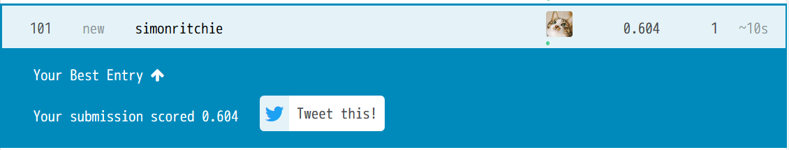
とりあえず、本日の作業分で、スコアは0.604(101/178)でした。まだ色々仮の状態ですが、それにしては意外と良い結果・・