bokehの対話的プロットを極力丁寧に理解するために、手頃なサンプルを例に解読を試みる。
ソースコードから予想で仕様を書いているが、ドキュメントも確認しているので大まかには間違いないはず。
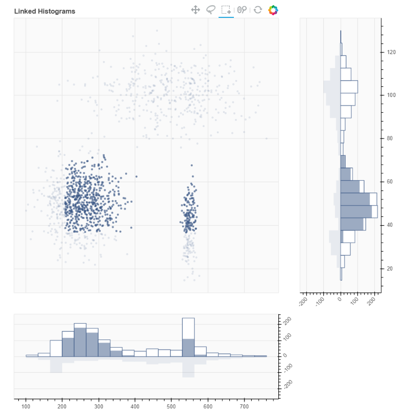
全体のソースコードはこちら
こんなやつ↓
データ生成
# create three normal population samples with different parameters
x1 = np.random.normal(loc=5.0, size=400) * 100
y1 = np.random.normal(loc=10.0, size=400) * 10

x2 = np.random.normal(loc=5.0, size=800) * 50
y2 = np.random.normal(loc=5.0, size=800) * 10

x3 = np.random.normal(loc=55.0, size=200) * 10
y3 = np.random.normal(loc=4.0, size=200) * 10

x = np.concatenate((x1, x2, x3))
y = np.concatenate((y1, y2, y3))
bokeh関係ないので説明は省略。
点群のプロット
TOOLS="pan,wheel_zoom,box_select,lasso_select,reset"

# create the scatter plot
p = figure(tools=TOOLS, plot_width=600, plot_height=600, min_border=10, min_border_left=50,
           toolbar_location="above", x_axis_location=None, y_axis_location=None,
           title="Linked Histograms")
p.background_fill_color = "#fafafa"
↑ figureオブジェクトに表示したいツールの名前を与え、背景色を設定。ここまでは普通のプロットと同じ流れ。
figureはbokeh.models.figureの関数でその返り値はbokeh.models.Figure。これに色々な設定を突っ込んでいく。
p.select(BoxSelectTool).select_every_mousemove = False
p.select(LassoSelectTool).select_every_mousemove = False
↑ このあたりから注意が必要。
まずp.select()はFigureのメソッドで、大本は継承元のbokeh.models.Modelのメソッド。
selectorのクラスオブジェクトを与えられると、figureに割り当てられている該当する種類のselectorを返す。
例えば一行目ではBoxSelectToolクラスのインスタンスが得られ、select_every_mousemoveをFalseにすることでマウス選択が完了するまではupdateが起きないように設定している。
リファレンス→
select(selector)
Query this object and all of its references for objects that match the given selector.
r = p.scatter(x, y, size=3, color="#3A5785", alpha=0.6)
ここで点群のプロット!返り値のrは最後に使う。
プロットしたときの返り値は一般にGlyphRendererクラスのインスタンスが返り、あとからプロットをいじるのに使える。
ヒストグラム
# create the horizontal histogram
hhist, hedges = np.histogram(x, bins=20)
hzeros = np.zeros(len(hedges)-1)
hmax = max(hhist)*1.1
↑ numpy.histrogram()の返り値は(各ヒストグラムの高さリスト, ヒストグラムの境界値リスト)。
bokehは関係ない。
LINE_ARGS = dict(color="#3A5785", line_color=None)

ph = figure(toolbar_location=None, plot_width=p.plot_width, plot_height=200, x_range=p.x_range,
            y_range=(-hmax, hmax), min_border=10, min_border_left=50, y_axis_location="right")
ph.xgrid.grid_line_color = None
ph.yaxis.major_label_orientation = np.pi/4
ph.background_fill_color = "#fafafa"

ph.quad(bottom=0, left=hedges[:-1], right=hedges[1:], top=hhist, color="white", line_color="#3A5785")
↑ 水平方向のヒストグラム。
設定項目がいよいよ多く煩雑だが、基本的な流れは変わらない。
figure()でFigureを取得して、それのquad()メソッドで四角形の描画を行っている。(ヒストグラム専用のメソッドではなく、座標に並行な四角形を描画するメソッドのようだ)。
bottom ~ top で4辺の座標指定をしている。
ひとつひとつの四角形はbokeh.models.glyphs.Quadクラスのインスタンスになるらしい。
それ以外の引数で便利そうなのは以下。
toolbar_location=None # ツールバー非表示
plot_width=p.plot_width # プロットの横幅の共有
x_range=p.x_range # x座標範囲の共有
min_border_left=50 # プロット左側の余白の最小値
ph.yaxis.major_label_orientation = np.pi/4 # 座標ラベルの回転
選択時のヒストグラム
つづいて点群を選んだときに表示されるヒストグラムだが、
hh1 = ph.quad(bottom=0, left=hedges[:-1], right=hedges[1:], top=hzeros, alpha=0.5, **LINE_ARGS)
hh2 = ph.quad(bottom=0, left=hedges[:-1], right=hedges[1:], top=hzeros, alpha=0.1, **LINE_ARGS)
なんと先に描いてしまっている。
この時点ではtop=hzerosなので高さ0に設定されており、見えないようになっている。
選んだときにこの返り値のhh1, hh2の高さが更新される、という仕組みなのだろう(※)。
鉛直方向のヒストグラム
# create the vertical histogram
vhist, vedges = np.histogram(y, bins=20)
vzeros = np.zeros(len(vedges)-1)
vmax = max(vhist)*1.1

pv = figure(toolbar_location=None, plot_width=200, plot_height=p.plot_height, x_range=(-vmax, vmax),
            y_range=p.y_range, min_border=10, y_axis_location="right")
pv.ygrid.grid_line_color = None
pv.xaxis.major_label_orientation = np.pi/4
pv.background_fill_color = "#fafafa"

pv.quad(left=0, bottom=vedges[:-1], top=vedges[1:], right=vhist, color="white", line_color="#3A5785")
vh1 = pv.quad(left=0, bottom=vedges[:-1], top=vedges[1:], right=vzeros, alpha=0.5, **LINE_ARGS)
vh2 = pv.quad(left=0, bottom=vedges[:-1], top=vedges[1:], right=vzeros, alpha=0.1, **LINE_ARGS)
水平方向と同じように設定がされている。
仕上げ
今までのものを組み上げる。
layout = gridplot([[p, pv], [ph, None]], merge_tools=False)
↑ まずbokeh.layouts.girdplot()関数でfigureを2次元的に並べている。ちなみに、2次元でなく縦または横に並べたいだけであればbokeh.layouts.columnまたはrowを使う。
curdoc().add_root(layout)
curdoc().title = "Selection Histogram"
↑ curdocはcurrent documentの略で、デフォルトのDocument(bokehの出力をまとめるクラス)を取得し、add_root()メソッドでグリッドと紐付けている。
ここが肝だが、「add_rootしたグリッドに何らかの変更が加わると、Documentに"on_change"で登録したコールバックが呼ばれる」、という仕様らしい。
リファレンスより→
add_root(model, setter=None)
Add a model as a root of this Document.
Any changes to this model (including to other models referred to by it) will trigger on_change callbacks registered on this document.
ということで先に最終行を見ると、
r.data_source.selected.on_change('indices', update)
としてたしかにon_changeにコールバックを登録している。
ここのrはscatter plot()の返り値(GlyphRendererクラスのインスタンス)で、
r.data_sourceはプロットしたデータセット、そのselectedはデータのうち選択された部分に相当する。
on_chage()はbokeh.model.Modelのメソッドで、そのオブジェクトにコールバックを登録する。
def on_change(self, attr, *callbacks):
        ''' Add a callback on this object to trigger when ``attr`` changes.

        Args:
            attr (str) : an attribute name on this object
            *callbacks (callable) : callback functions to register
第一引数attrが分かりづらいが、ここには「何が変化したらコールバックを呼ぶか」を記述する。今回は選択範囲(=データのインデックス=selection.indices)なので"indices"を指定している。
なお、変更ではなく特定のイベント(ボタンが押されるとか、スライダーが動かされるとか)にコールバックを結びつけたい場合は
on_event(event, callback)
を使う。
(以下余談)
ここではPythonの関数を登録しているが、javascriptで記述した関数(bokeh.models.CustomJSのインスタンス)を登録したければ
m.js_on_change(attr, callback)
を用いればよい。このあたりは公式チュートリアルの6章に記述がある。
単体のhtml出力がほしければこちらを使う必要があるらしい。
実行時のワーニング→
WARNING:bokeh.embed.util:
You are generating standalone HTML/JS output, but trying to use real Python
callbacks (i.e. with on_change or on_event). This combination cannot work.

Only JavaScript callbacks may be used with standalone output. For more
information on JavaScript callbacks with Bokeh, see:

    https://docs.bokeh.org/en/latest/docs/user_guide/interaction/callbacks.html

Alternatively, to use real Python callbacks, a Bokeh server application may
be used. For more information on building and running Bokeh applications, see:

    https://docs.bokeh.org/en/latest/docs/user_guide/server.html
(余談ここまで)
最後にコールバック関数update()の中身について、
def update(attr, old, new):
    inds = new
    if len(inds) == 0 or len(inds) == len(x):
        hhist1, hhist2 = hzeros, hzeros
        vhist1, vhist2 = vzeros, vzeros
    else:
        neg_inds = np.ones_like(x, dtype=np.bool)
        neg_inds[inds] = False
        hhist1, _ = np.histogram(x[inds], bins=hedges)
        vhist1, _ = np.histogram(y[inds], bins=vedges)
        hhist2, _ = np.histogram(x[neg_inds], bins=hedges)
        vhist2, _ = np.histogram(y[neg_inds], bins=vedges)

    hh1.data_source.data["top"]   =  hhist1
    hh2.data_source.data["top"]   = -hhist2
    vh1.data_source.data["right"] =  vhist1
    vh2.data_source.data["right"] = -vhist2
引数にはon_changeで指定したattrと、その属性の変化前後の値old, newが与えられるようだ。
ここではnewが新しく選択した点群のインデックスということになる。
(※)の予言の通り、選ばれたインデックスに応じて水平方向ヒストグラムのtopの値が更新されている。
参照関係がちょっと遠いが、
もとのデータセット
↑
scatter plot (=水平方向ヒストグラムとデータソースを共有)
↑
selection
↑
on_changeコールバック
のような感じでつながっているのでon_changeの引数に与えられるインデックスは最初のデータセットのインデックスと同一であることがわかる。