はじめに
”カオス(Chaos)”の響きはとてもそそられるものがあります。バタフライエフェクトなど、有名なキーワードもカオスの研究分野から生まれています。カオスについて少しかじってみる機会がありましたので、本記事ではカオスな挙動を生み出す数々の方程式と、それらのpythonを使った観察についてご紹介したいと思います!
カオスとは?
カオスとは、「最初の状態がほんの少し違うだけで、将来非常に大きな違いを生む」という初期値に対する鋭敏性が最も大きな特徴です1。カオスの生まれる源は確率的な概念ではなく、初期値とパラメータによって時間発展が完全に記述できるハズの方程式でありながも、僅かな初期値の違いによっても長期的な解の挙動が大きく異なる(不確定性が指数的に増大する)事にあります。すなわち、時間$t$後において、系の不確定性 $N(t)$が $N(t)=\exp(\lambda t)$となります。ここで$\lambda>0$はLiapnov exponentと呼ばれる定数で、系の不確定性の増大の程度を示しています。2 長期的な天気予報を正確に行う事が困難であることも、この初期値の僅かな違いによって生じる大きな系の不確定性に由来しています。3また、解が非周期的で予測が困難であることもカオスな系の特徴として挙げられます。
バタフライ・エフェクト
「バタフライ・エフェクト」は、非常に有名となっています。すなわち、「蝶のはばたきが、トルネードを巻き起こす」といった内容です。すなわち気象モデルなどカオスを含む系では、蝶のはばたきの様なほんの僅かな初期値の違いですら、長期的には大きな影響が生じる可能性がある(“sensitive dependence on initial conditions”)という事です。4 では、一体カオスとはどんな姿をしているのでしょうか?
カオスな微分方程式
カオスな挙動が見られる一例として、減衰ありの強制振動を記述する微分方程式の一例であるDuffing's equationを見てみましょう。係数の値については、"An introduction to differential equations and their applications" (Stanley J. Farlow, 1994)のものを参考としています。
一般式:
\ddot{x}+\delta \dot{x}+\alpha x+\beta x^3=\gamma \cos(\omega t)\\
J. Farlow\ (1994):
\ddot{x}+0.05\dot{x}+x^3=7.5x
これは単純な微分方程式に見えますが、非線形項の存在によってカオスな挙動を示します。僅かに異なる初期値を与えて、位相空間における解の挙動を見てみましょう。以下のコードでは、$\dot{x}=y$とおいて二階の微分方程式を一階の連立微分方程式へと変換し、それらを数値的に解いています。
import numpy as np
import matplotlib.pyplot as plt
def forward(x,y,i,h):
        x_i=x
        y_i=y

        x_iplus1=x_i+h*y_i
        y_iplus1=y_i+h*(-0.05*y_i-x_i**3+7.5*np.cos(i*h))

        return x_iplus1,y_iplus1

iteration=20000
h=0.001

x_0_1=3
y_0_1=4
x_1=[x_0_1]
y_1=[y_0_1]

x_0_2=3.01
y_0_2=4.01

x_2=[x_0_2]
y_2=[y_0_2]

for i in range(iteration):
    x_iplus1,y_iplus1=forward(x_1[i],y_1[i],i,h)
    x_1.append(x_iplus1)
    y_1.append(y_iplus1)

    x_iplus1,y_iplus1=forward(x_2[i],y_2[i],i,h)
    x_2.append(x_iplus1)
    y_2.append(y_iplus1)

fig=plt.figure(figsize=(10,4))
ax=fig.subplots()
ax.plot(x_1,y_1,label="(3,4)")
ax.plot(x_2,y_2,label="(3.1,4.1)")
ax.set_xlabel("x",fontsize=20)
ax.set_ylabel("$\dot{x}$",fontsize=20)
ax.set_ylim(-6,8)
ax.legend()
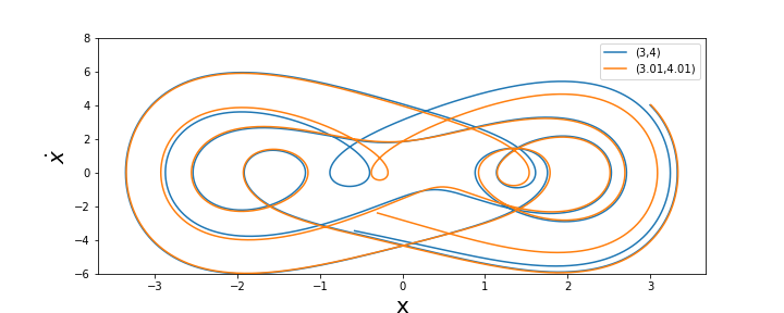
出力された結果を見ると、僅か0.01の差の初期値の差だったにも関わらず、時間が経つにつれて差が拡大している様子が観察できます。これは初期値に対する鋭敏性を表す一例です。
カオスな系とストレンジアトラクター
どんどんと微分方程式の計算を進めていくと、一定の決まった値へと収束したり、周期的に解が振動する場合があります。それでは、カオスな系では時間発展の結果はどの様になるのでしょうか?この場合には従来のアトラクターではなく、ストレンジアトラクターと呼ばれる概念が登場します。自分の理解としては、系が時間発展するにつれて多くの解がその周囲に集まる最小の領域の集合がストレンジアトラクターですが、詳細な数学的理論についてはよく理解していないので割愛させてください。先ほどのDuffing's equationの軌道上に一定の時間間隔($\frac{2\pi}{\omega}$)で点を打ち、それらの挙動を見てみましょう。今度のパラメータは、このサイトを参考としています。
\ddot{x}+0.1\dot{x}-x+x^3=0.35\cos(1.4t)
from tqdm import tqdm
iteration=100000000
h=0.0005
x_0=0
y_0=0
x=[x_0]
y=[y_0]

def forward(x,y,i,h):
        x_i=x
        y_i=y

        x_iplus1=x_i+h*y_i
        y_iplus1=y_i+h*(x_i-x_i**3-0.1*y_i+0.35*np.cos(1.4*i*h))

        return x_iplus1,y_iplus1

for i in tqdm(range(iteration)):
    x_iplus1,y_iplus1=forward(x[i],y[i],i,h)
    x.append(x_iplus1)
    y.append(y_iplus1)

fig=plt.figure(figsize=(15,10))
ax=fig.subplots()
omega=1.4

max=int(iteration*h/(2*np.pi/omega))

x_points=[x[int((2*np.pi*i/omega)/h)] for i in range(max)]
y_points=[y[int((2*np.pi*i/omega)/h)] for i in range(max)]

ax.scatter(x_points,y_points,s=3)

ax.set_xlabel("x",fontsize=20)
ax.set_ylabel("$\dot{x}$",fontsize=20)
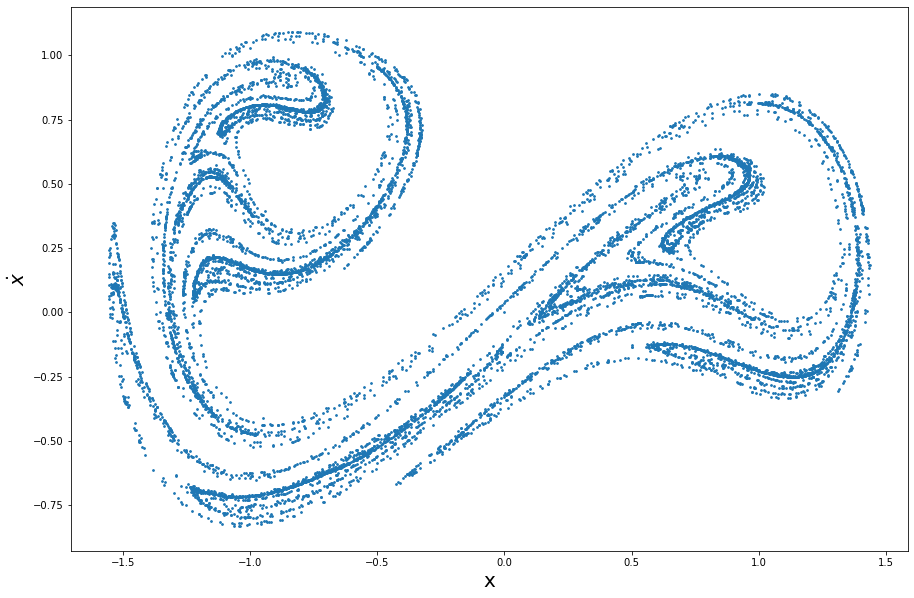
カオス感じますね!!
この図はPoincaré map(またはPoincaré section)と呼ばれ、ストレンジアトラクターを見えやすくする為に5、系へ加わる外力の周期ごとにサンプリングを行った結果を図示したものです。これによって、連続的な微分方程式の解を離散的に代表することが可能となります2。ちなみにですが、ストレンジアトラクターは一部を拡大しても、拡大前と同様の形状が生じる自己相関性(フラクタル)の性質を持つことが知られています。
シンプルな二階の微分方程式からも、興味深い挙動が生じる事が分かりました。以下では、カオスな解が生じる有名な方程式について、コードと共に見ていきたいと思います!
ロジスティック写像
ロジスティック写像は以下の式で表現される極めて単純な式をしており、パラメータも$a$の一つしかありません。しかしながら、そこから生じる解の挙動は非常に面白いものとなっています!
x_{n+1}=ax_n(1-x_n)
ロジスティック写像が出現する例としては、例えば生物の個体数のモデリングが挙げられます。すなわち、次年度の個体数(正確には最大の個体数に占める割合ですが)$x_{n+1}$は前年度の個体数 $x_n $と、環境収容力$1-x_n$の積に比例するという考え方です。$a$の値に対する$x_n$の挙動を見るため、ロジスティック写像を計算し、$x_n$がどの様に極限値へ近づいていくのかを描画してみましょう。ここで極限値の判定には5000階級のヒストグラムを使い、5個以上の$x_n$を含む階級値を収束値の代表として採用しています。また、初期値は0~1の範囲でランダムに選択しています。
import numpy as np
import matplotlib.pyplot as plt
from mpl_toolkits.mplot3d import axes3d
from matplotlib.animation import FuncAnimation
from tqdm import tqdm

a=0.95 #パラメータ
iterate=500 #繰り返し数

def logistic_map(a):
    x_n=x_0
    values=[x_n]
    for i in range(iterate):
        x_n=a*x_n*(1-x_n)
        values.append(x_n)
    return values

def limitValueFinder(logistic_mapp,a,listOfXcoords,listOfYcoords):
    output=logistic_map(a)
    n,bins=np.histogram(output,5000)
    limitValueLocations=np.where(n>5)[0]
    limitValues=[bins[loc] for loc in limitValueLocations]
    listOfXcoords.extend([a for i in range(len(limitValueLocations))])
    listOfYcoords.extend(limitValues)
    return listOfXcoords, listOfYcoords

x_0=np.random.uniform(0,1)

values=logistic_map(a)
x_n=values[:-1]
x_n_plus_1=values[1:]

listOfXcoords=[]
listOfYcoords=[]
_,limitY=limitValueFinder(logistic_map,a,listOfXcoords,listOfYcoords)

fig=plt.figure(figsize=(10,10))
ax=fig.subplots(2)
ax1=ax[0]
ax1.scatter(x_n,x_n_plus_1,s=30)
ax1.scatter(limitY,[a*limValue*(1-limValue) for limValue in list(limitY)],s=15,color="red",label=f"Limit at: a={a}, iteration={iterate}")
ax1.set_xlabel("$x_n$",fontsize=13)
ax1.set_ylabel("$x_{n+1}$",fontsize=13)
ax1.legend()

ax2=ax[1]
ax2.scatter([i for i in range(len(values))],values,s=20)
ax2.scatter([iterate for i in range(len(limitY))],limitY,s=10,color="red",label=f"Limit at: a={a}, iteration={iterate}")
ax2.set_xlabel("n",fontsize=13)
ax2.set_ylabel("x_n",fontsize=13)
ax2.legend(fontsize=15)

こちらの図を見ると、値が0へと収束していく様子が分かります。この性質は$0<a<1$の条件の下で、一般に成立しています。それでは、0より大きな$a$では収束値は一体どうなっているのでしょうか?$a$の値を変化させて、その様子を見てみましょう。今回は収束の過程は重要ではない為、最初から100番目までの$x_n$の値は除いています。
from matplotlib.animation import FuncAnimation

x_0=np.random.uniform(0,1)

fig=plt.figure(figsize=(15,10))
ax=fig.subplots()

iterate=30000
def logistic_map(a):
    x_n=x_0
    values=[x_n]
    for i in range(iterate):
        x_n=a*x_n*(1-x_n)
        values.append(x_n)
    values=np.delete(values,slice(0,100))
    return values

def update(frame):
    ax.cla()

    Ulimit=frame

    listOfXcoords=[]
    listOfYcoords=[]

    A=np.linspace(0,Ulimit,200)
    for a in A:
        limitValueFinder(logistic_map,a,listOfXcoords,listOfYcoords)
        ax.scatter(listOfXcoords,listOfYcoords,s=0.01,color="black")
    ax.set_xlim([0,4])
    ax.set_ylim([0,1])

anim=FuncAnimation(fig,update,frames=np.linspace(0.1,3.999,30),interval=500)
anim.save("Logistic_map.gif",writer="imagemagick")

$a$の値を変化させていくと、解の挙動が劇的に変化する個所が存在します。実際には$3.5699456...<a<4$の範囲では値は収束しておらず、非周期的な挙動のカオスが出現しています。こちらの範囲のみを拡大して、詳しく観察してみましょう。
fig=plt.figure(figsize=(10,10))
ax=fig.subplots()
listOfXcoords=[]
listOfYcoords=[]

start=3.5699456
end=3.99999
ticks=2000
A=np.linspace(start,end,ticks)
for a in A:
    limitValueFinder(logistic_map,a,listOfXcoords,listOfYcoords)
ax.scatter(listOfXcoords,listOfYcoords,s=0.00005,color="black")
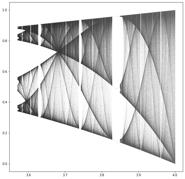
とても複雑かつ美しい値の分布が観察できます。この領域は全てがカオスなのではなく、すっぽりと抜けている個所(窓領域)では、解が周期的な軌道へと戻っています。窓領域で観察される周期軌道は$a<3.5699456$の範囲で観察できる周期軌道とは異なる原因で生じているらしいですが、数学的な詳細を存じ上げない為、省略致します。
ロジスティック写像のまとめとしまして、各$a$の値による解の性質について以下に概要と、各領域毎に色分けをした分岐図を掲載しました。解の性質については、"An introduction to differential equations and their applications" (Stanley J. Farlow, 1994)に概ね基づいています。
①$0<a<1$
$x_n$は0へ収束します。
②$1<a\leqq3$
$x_n$は$\frac{a-1}{a}$へと収束します。
③$3<a\leqq3.4495$
$x_n$は単一の点へと収束するのではなく、2つの値の間をジャンプするようになります。(bifurcation)
④$3.4495<a\leqq3.56...$
$x_n$のジャンプする数は4、8、16、32…の様に増大していきます。
⑤$3.56...<a<4$
カオスな挙動が見られる様になります。
fig=plt.figure(figsize=(20,10))
ax=fig.subplots()

x_0=np.random.uniform(0,1)

iterate=30000

def logistic_map(a):
    x_n=x_0
    values=[x_n]
    for i in range(iterate):
        x_n=a*x_n*(1-x_n)
        values.append(x_n)
    values=np.delete(values,slice(0,100))
    return values

# 0<a<=1
listOfXcoords=[]
listOfYcoords=[]

start=0.001
end=1.0
ticks=1000
A=np.linspace(start,end,ticks)
for a in tqdm(A):
    limitValueFinder(logistic_map,a,listOfXcoords,listOfYcoords)
ax.scatter(listOfXcoords,listOfYcoords,s=0.1,color="blue",label="0<a<=1")

# 1<a<=3
listOfXcoords=[]
listOfYcoords=[]

start=1
end=3
ticks=1000
A=np.linspace(start,end,ticks)
for a in tqdm(A):
    limitValueFinder(logistic_map,a,listOfXcoords,listOfYcoords)
ax.scatter(listOfXcoords,listOfYcoords,s=0.1,color="green",label="1<a<=3")

# 3<a<=3.4494897...
listOfXcoords=[]
listOfYcoords=[]

start=3
end=3.4494987
ticks=1000
A=np.linspace(start,end,ticks)
for a in tqdm(A):
    limitValueFinder(logistic_map,a,listOfXcoords,listOfYcoords)
ax.scatter(listOfXcoords,listOfYcoords,s=0.1,color="red",label="3<a<=3.4494897..")

# 3.4494897...<a<=3.5699456...
listOfXcoords=[]
listOfYcoords=[]

start=3.4494987
end=3.5699456
ticks=1000
A=np.linspace(start,end,ticks)
for a in tqdm(A):
    limitValueFinder(logistic_map,a,listOfXcoords,listOfYcoords)
ax.scatter(listOfXcoords,listOfYcoords,s=0.001,color="cyan",label="3.4494897...<a<=3.5699456...")

# 3.5699456...<a<4
listOfXcoords=[]
listOfYcoords=[]

start=3.5699456
end=3.99999
ticks=2000
A=np.linspace(start,end,ticks)
for a in tqdm(A):
    limitValueFinder(logistic_map,a,listOfXcoords,listOfYcoords)
ax.scatter(listOfXcoords,listOfYcoords,s=0.000005,color="black",label="3.5699456...<a<4")

ax.set_xlabel("a", fontsize=13)
ax.set_ylabel("Limit",fontsize=13)

ax.legend(fontsize=15)
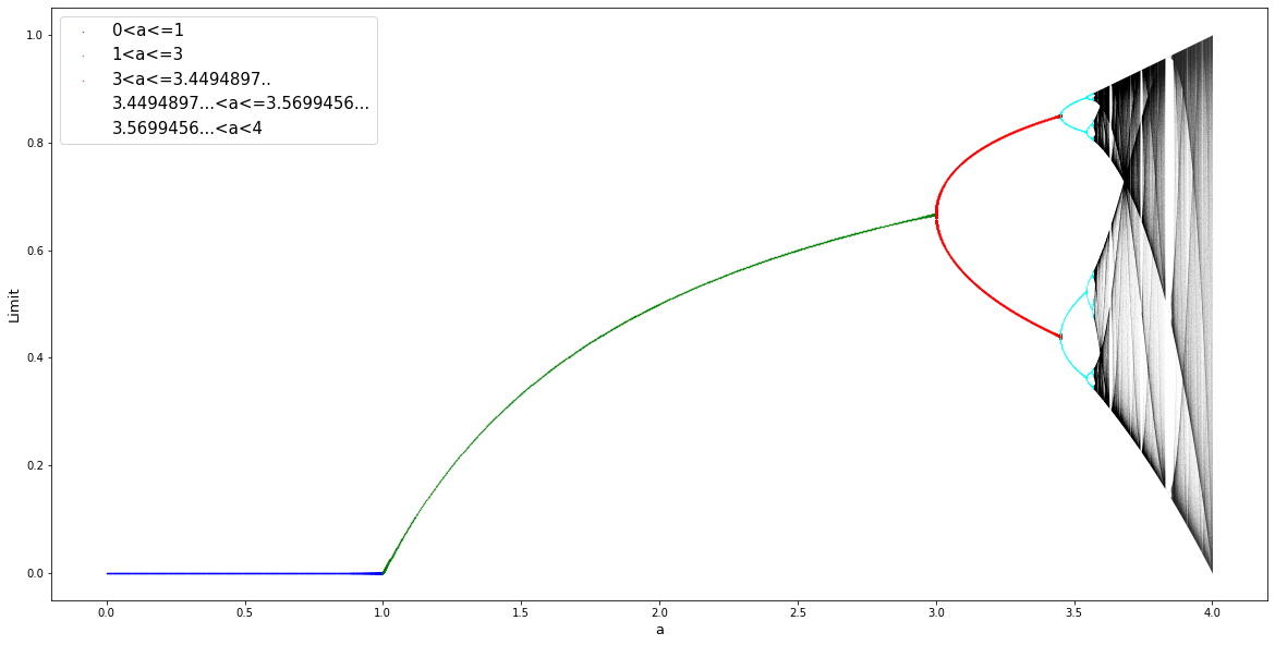
色分けによって、各領域での解の様子の違いが見やすくなったかな…と思います。こちらのロジスティック写像ですが、マンデルブロ集合と立体的に結びついていることが知られています。6 シンプルな数列から生まれた図形が複素平面の概念と結びついてるのは、とても面白いと感じました。
ローレンツ方程式
1963年にMITの気象学者であったEdward Lorenzは熱対流する大気の挙動を記述する以下の非線形な微分方程式を用いて研究を行っていました。初期条件を小数点以下6桁の精度で計算を行った後、初期条件を小数点以下3桁の精度で改めて計算したところ、その結果は一回目と大きく違って表示されていました。このカオスな系に特有な初期値への敏感さを受けて、Lorenzは「もし現実の大気がこの様にふるまうのならば、長期的な天気の予測は不可能と思っていました("I knew that if the real atmosphere behaved like this [mathematical model], long-range weather prediction was impossible")」とDiscover magazineへ語ったとされています。2
\dot{x}=-10x+10y\\
\dot{y}=28x-y+xz\\
\dot{z}=-\frac{8}{3}z+xy
それでは、pythonを使って実際のローレンツ方程式の解の挙動を見てみましょう。
import numpy as np
import matplotlib.pyplot as plt
from mpl_toolkits.mplot3d import axes3d
from matplotlib.animation import FuncAnimation
from tqdm import tqdm

p=10
r=28
b=8/3
h=0.001

x_0=5
y_0=5
z_0=5

def forward(x,y,z,p,r,b,h):
    x_i=x
    y_i=y
    z_i=z

    x_iplus1=x_i-h*p*x_i+h*p*y_i
    y_iplus1=y_i-h*x_i*z_i+r*h*x_i-h*y_i
    z_iplus1=z_i+h*x_i*y_i-b*h*z_i

    return x_iplus1,y_iplus1,z_iplus1

iterate=50000
x=[x_0]
y=[y_0]
z=[z_0]

for i in tqdm(range(iterate)):
    x_iplus1_j,y_iplus1_j,z_iplus1_j=forward(x[i],y[i],z[i],p,r,b,h)
    x.append(x_iplus1_j)
    y.append(y_iplus1_j)
    z.append(z_iplus1_j)

plt.style.use('ggplot')
plt.rcParams["axes.facecolor"] = 'white'

fig = plt.figure(figsize=(10,10))
ax = fig.gca(projection='3d')

ax.plot(x, y, z, label='Lorentz curve')
ax.legend()
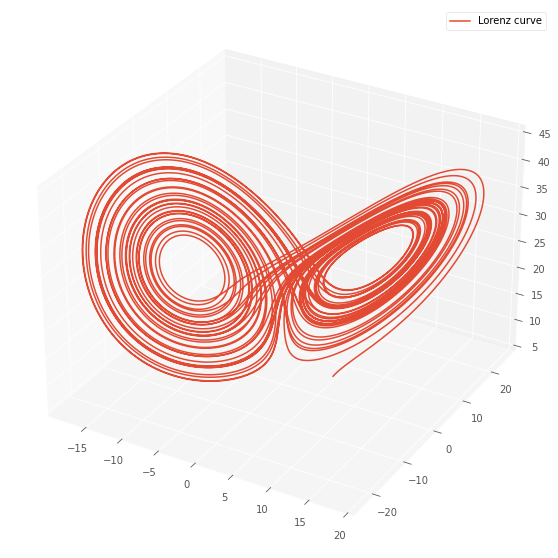
非常に有名なローレンツ方程式の解の図が描画出来ました。蝶の様な二つのアトラクターの間で、解がジャンプしている様子が観察できます。エネルギー保存と熱保存の二つの保存量の値が系に含まれる非保存的な項の作用によって変化し、特定の条件の下で別の状態へと遷移することが、この特徴的なジャンプの理由とされています。7
それでは、初期値やローレンツ方程式のパラメータを変える事で、どの様に解の挙動が変わるのかを見てみましょう!まずは初期値を0から5まで、約0.05刻みで変化させた場合です。
p=10
r=28
b=8/3
h=0.001

plt.style.use('ggplot')
plt.rcParams["axes.facecolor"] = 'white'

fig = plt.figure(figsize=(10,10))
ax = fig.gca(projection='3d')

def update(frame):
    ax.cla()

    x_0=frame
    y_0=frame
    z_o=frame

    iterate=50000

    x=[x_0]
    y=[y_0]
    z=[z_0]


    for i in range(iterate):
        x_iplus1_j,y_iplus1_j,z_iplus1_j=forward(x[i],y[i],z[i],p,r,b,h)
        x.append(x_iplus1_j)
        y.append(y_iplus1_j)
        z.append(z_iplus1_j)

    ax.plot(x, y, z, label=f'x_0=y_0=z_0={frame:.2f}')
    ax.legend()

anim=FuncAnimation(fig,update,frames=np.linspace(0.1,5,100),interval=200)
anim.save("Lorentz_2.gif",writer="imagemagick")
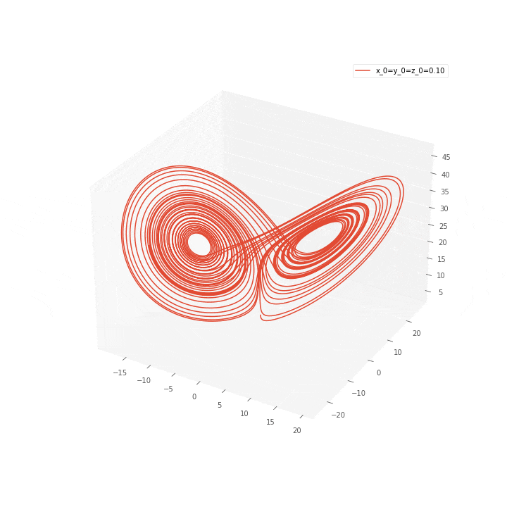
ジャンプが生じる場所は初期値を変えてもあまり影響されていませんが、解の形状は初期値へ鋭敏に反応している様子が分かります。
次に、一部のパラメータを変更して形状の変化を見てみましょう。ローレンツ方程式のうち、$\dot{y}$についての式中の$x$の係数をパラメータ$r$として、その変化による解の挙動を観察してみます。
p=10
b=8/3
h=0.001

plt.style.use('ggplot')
plt.rcParams["axes.facecolor"] = 'white'

fig = plt.figure(figsize=(10,10))
ax = fig.gca(projection='3d')

def update(frame):
    ax.cla()

    r=frame

    x_0=5
    y_0=5
    z_o=5

    iterate=50000

    x=[x_0]
    y=[y_0]
    z=[z_0]

    for i in range(iterate):
        x_iplus1_j,y_iplus1_j,z_iplus1_j=forward(x[i],y[i],z[i],p,r,b,h)
        x.append(x_iplus1_j)
        y.append(y_iplus1_j)
        z.append(z_iplus1_j)

    ax.plot(x, y, z, label=f'r={frame:.2f}')
    ax.legend()

anim=FuncAnimation(fig,update,frames=np.linspace(0.1,145,100),interval=200)
anim.save("Lorentz_3.gif",writer="imagemagick")

このパラメータをした場合にも、いくつか興味深い変化が生じています。$r$が20程度までは、解は一点に収束している様に見えます。$r$を増大すると、先ほどの蝶の様な形が見られる様になりますが、$r$を更に増していくと形が崩れてしまいます。
3種の生物による競争方程式
ロトカ・ヴォルテラ方程式は生態系における個体数変動などを追跡する為の連立微分方程式です。捕食者と被食者の間(二種)についての研究は広く行われ、その挙動はよく知られているものの、3種まで拡張した場合には現在も研究が進行するホットなテーマとなっています。8
今回用いるのは、こちらの論文'Hastings, Alan, and Thomas Powell. "Chaos in a three‐species food chain." Ecology 72.3 (1991): 896-903.'中で扱われている3種の生物による競争方程式です。支配方程式は、以下の通りです。ここで、$x$は食物連鎖中で最下位の生物、$y$は中間、$z$は最上位の生物を表しています。
\frac{dx}{dt}=x(1-x)-f_1(x)y\\
\frac{dy}{dt}=f_1(x)y-f_2(y)z-d_1y\\
\frac{dz}{dt}=f_2(y)z-d_2z\\
*f_i(u)=\frac{a_iu}{1+b_iu}
では、pythonで実装していきましょう。パラメータの値については、論文中で紹介されているものを使用しました。
import numpy as np
import matplotlib.pyplot as plt
from mpl_toolkits.mplot3d import axes3d
from matplotlib.animation import FuncAnimation
from tqdm import tqdm

a1=5
b1=3
a2=0.1
b2=2
d1=0.4
d2=0.01

h=0.01

x_0=0.75
y_0=0.18
z_0=9.9

def f(u,a,b):
    return a*u/(1+b*u)

def forward(x,y,z,h):
    x_i=x
    y_i=y
    z_i=z

    x_iplus1=x_i+h*(x_i*(1-x_i)-f(x_i,a1,b1)*y_i)
    y_iplus1=y_i+h*(f(x_i,a1,b1)*y_i-f(y_i,a2,b2)*z_i-d1*y_i)
    z_iplus1=z_i+h*(f(y_i,a2,b2)*z_i-d2*z)

    return x_iplus1,y_iplus1,z_iplus1

iterate=300000
x=[x_0]
y=[y_0]
z=[z_0]

for i in tqdm(range(iterate)):
    x_iplus1_j,y_iplus1_j,z_iplus1_j=forward(x[i],y[i],z[i],h)
    x.append(x_iplus1_j)
    y.append(y_iplus1_j)
    z.append(z_iplus1_j)
上記のコードによって個体数の計算が終わったので、結果を図示していきましょう。まずは、個々の生物の個体数増減を別々に表示してみます。
fig=plt.figure(figsize=(8,10))
ax=fig.subplots(3)
ax1=ax[0]
ax1.plot(x)
ax2=ax[1]
ax2.plot(y)
ax3=ax[2]
ax3.plot(z)

ax1.set_xlim(0,150000)
ax1.set_ylabel("x",fontsize=20)
ax2.set_xlim(0,150000)
ax2.set_ylabel("y",fontsize=20)
ax3.set_xlim(0,150000)
ax3.set_ylabel("z",fontsize=20)

一見周期的に見えますが、細部を見ると毎回の繰り返しが微妙に形が変わっているのが観察できます(カオスの非周期性)。次に、個体数の変動を3次元プロットで表示してみましょう。
plt.style.use('ggplot')
plt.rcParams["axes.facecolor"] = 'white'

fig = plt.figure(figsize=(10,10))
ax = fig.gca(projection='3d')

ax.plot(x, y, z, label='Lotka-Volterra 3 species')
ax.set_ylim([np.max(y),np.min(y)])
ax.set_xlabel("x",fontsize=20)
ax.set_ylabel("y",fontsize=20)
ax.set_zlabel("z",fontsize=20)
ax.legend()
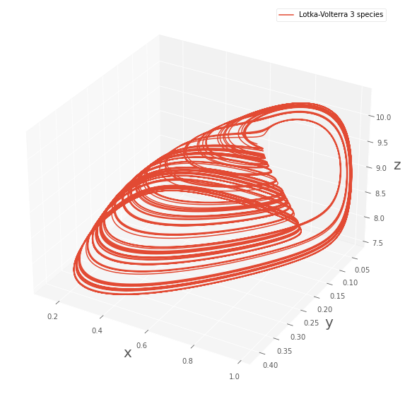
なんだか面白い形が出てきました!論文中の説明によれば、系は時間発展するにつれて3次元プロット(tea cupと形容されています)の上から垂れている細い領域を下に降りていき、広い領域を下から上に向かって遷移した後、再び細い領域へ入ります。
すなわち、大きくは”頂点捕食者zが減る→下位の動物が増加する→食料増加でzが増える→yが食われて数を減らす→食料不足でzの数が減る”のサイクルを繰り返しています。しかしながら、決して一つの定常的な軌道に収束はしていないことが特徴です。また、ティーカップの柄の部分では多くの軌道が接近しているため、この点における僅かな測定値の違いが将来的には大きな違いとして出てきます(カオスな系の初期値への鋭敏性)。
おまけ(鳥の形のストレンジアトラクター)
こちらのサイトにて紹介されていた鳥に似た形状が生じるアトラクターが興味深かったので、最後にpythonコードと共にご紹介致します。
x_{n+1}=y_n-0.97x_n+\frac{5}{1+(x_n)^2}-5\\
y_{n+1}=-0.995x_n
import numpy as np
import matplotlib.pyplot as plt
from tqdm import tqdm

iteration=1000000
h=0.001

x_0=1
y_0=0

x=[x_0]
y=[y_0]

def forward(x,y,h):
        x_i=x
        y_i=y

        x_iplus1=y_i-0.97*x_i+5/(1+x_i**2)-5
        y_iplus1=-0.995*x_i

        return x_iplus1,y_iplus1

for i in tqdm(range(iteration)):
    x_iplus1,y_iplus1=forward(x[i],y[i],h)
    x.append(x_iplus1)
    y.append(y_iplus1)

fig=plt.figure(figsize=(10,4))
ax=fig.subplots()
ax.scatter(x,y,s=0.01,color="black")
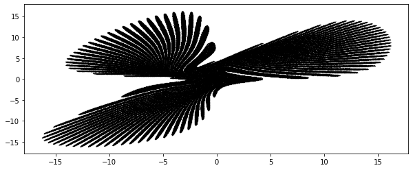
鳥さん🐤🐤🐤🐤🐤🐤🐤🐤🐤🐤🐤🐤🐤🐤🐤🐤🐤🐤🐤🐤
おわりに
純粋な興味関心から触れてみたカオスの世界ですが、フラクタルとのつながりや、単純な数式から複雑な形が形成できるなど、非常に興味深い内容が多かったです。カオスを巡る分野は今後更に発展していくと思いますので、これからどんな面白い概念が出てくるのかとても楽しみです!最後に、ここまで読んでいただき、本当にありがとうございました。また機会がありましたら、記事にお目を通して頂けると嬉しいです🐤
カオスについての面白いビデオのご紹介
"Chaos: The Science of the Butterfly Effect"
*筆者は数学を専門で学んでいない為、数学的に怪しい記述も多々見受けられたと思います。不正確な個所につきましては修正を行いますので、コメントを頂けますと幸いです。どうぞよろしくお願い致します。
-
Stanley J. Farlow: "An introduction to differential equations and their applications", Dover publications, 1994 ↩ ↩2 ↩3
-
MIT technology review: "When the Butterfly Effect Took Flight" ↩
-
James Gleick: "Chaos", penguin books, 2008 ↩
-
This equation will change how you see the world (the logistic map) ↩
-
[町田憲彦, 細野雄三. "3 種ロトカ・ボルテラ競争系の共存解の安定性と特異摂動解析." 京都産業大学論集. 自然科学系列 33 (2004): 23-44.] ↩