StanとRでベイズ統計モデリング(アヒル本)をPythonにしてみる - 11.4 Latent_Dirichlet_Allocation

実行環境

インポート

import numpy as np
import pandas as pd
import pystan
import matplotlib.pyplot as plt
from matplotlib.figure import figaspect
from matplotlib import gridspec
import seaborn as sns
%matplotlib inline

データ読み込み

lda = pd.read_csv('./data/data-lda.txt')

11.4 Latent_Dirichlet_Allocation

11.4.1 解析の目的とデータの分布の確認

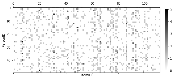
書籍のほうでは散布図を使っていますが、crosstabの後にmeltしてとか面倒くさかったので隙間のせいで偏った印象を与えないようにmatshowを使いました。

im = plt.matshow(pd.crosstab(lda['PersonID'], lda['ItemID']), cmap='binary', aspect='equal')
plt.colorbar(im, fraction=0.02, pad=0.03)
plt.setp(plt.gca(), xlabel='ItemID', ylabel='PersonID')
plt.show()

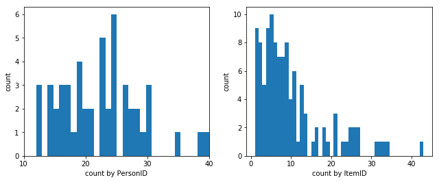
_, (ax1, ax2) = plt.subplots(1, 2, figsize=figaspect(3/8))
ax1.hist(lda.groupby('PersonID').count().unstack(), bins=30)
plt.setp(ax1, xticks=np.arange(10, 41, 10), xlim=(10, 40), xlabel='count by PersonID', ylabel='count')
ax2.hist(lda.groupby('ItemID').count().unstack(), bins=45)
plt.setp(ax2, xlabel='count by ItemID', ylabel='count')
plt.show()

11.4.4 Rでシミュレーション

N = 50
I = 120
K = 6

np.random.seed(123)
alpha0 = np.full(K, 0.8)
alpha1 = np.full(I, 0.2)
theta = np.random.dirichlet(alpha0, N)
phi = np.random.dirichlet(alpha1, K)

num_items_by_n = np.round(np.exp(np.random.normal(2.0, 0.5, N))).astype(int)

d = pd.DataFrame()
for n in range(N):
    z = np.random.choice(np.arange(K), num_items_by_n[n], replace=True, p=theta[n])
    item = [np.random.choice(np.arange(I), 1, replace=True, p=phi[k])[0] for k in z]
    d = d.append(pd.DataFrame(dict(PersonID=np.repeat(n, len(item)), ItemID=item)))

11.4.5 Stanで実装

K = 6
N = lda['PersonID'].max()
I = lda['ItemID'].max()
data = dict(
    E=lda.index.size,
    N=N,
    I=I,
    K=K,
    PersonID=lda['PersonID'],
    ItemID=lda['ItemID'],
    Alpha=np.repeat(0.5, I)
)
stanmodel = pystan.StanModel('./stan/model11-8.stan')
# fit_nuts = stanmodel.sampling(data=data, seed=123)
fit_vb = stanmodel.vb(data=data, seed=123)

ms = pd.read_csv(fit_vb['args']['sample_file'].decode('utf-8'), comment='#')

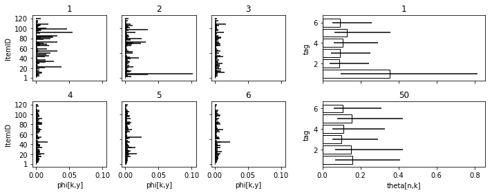
probs = (10, 25, 50, 75, 90)
idx = np.array([[k+1, i+1] for k, i in np.ndindex(K, I)])

d_qua = np.array([np.percentile(ms['phi.{}.{}'.format(k, i)], probs) for k, i in idx])
d_qua = pd.DataFrame(np.hstack((idx, d_qua)), columns=['tag', 'item']+['p{}'.format(p) for p in probs])

fig = plt.figure(figsize=figaspect(2/5))
gs1 = gridspec.GridSpec(2, 3)
for i, pos in enumerate(np.ndindex(2, 3)):
    ax = fig.add_subplot(gs1[pos], sharex=ax if i > 0 else None)
    ax.hlines('item', 0, 'p50', data=d_qua.query('tag==@i+1'))
    if pos[0] == 0:
        plt.setp(ax.get_xticklabels(), visible=False)
    else:
        plt.setp(ax, xlabel='phi[k,y]')
    if pos[1] == 0:
        plt.setp(ax, yticks=[1] + list(np.arange(20, 121, 20)), ylabel='ItemID')
    else:
        plt.setp(ax.get_yticklabels(), visible=False)
    plt.setp(ax, title=i+1)
gs1.tight_layout(fig, rect=[None, None, 0.6, None])

idx = np.array([[n+1, k+1] for n, k in np.ndindex(N, K)])

d_qua = np.array([np.percentile(ms['theta.{}.{}'.format(n, k)], probs) for n, k in idx])
d_qua = pd.DataFrame(np.hstack((idx, d_qua)), columns=['person', 'tag']+['p{}'.format(p) for p in probs])

gs2 = gridspec.GridSpec(2, 1)
for i, person in enumerate([1, 50]):
    ax = fig.add_subplot(gs2[i], sharex=ax if i > 0 else None)
    sub = d_qua.query('person==@person')
    ax.barh('tag', 'p50', data=sub, xerr=(sub['p25'], sub['p75']), color='w', edgecolor='k')
    if i == 0:
        plt.setp(ax.get_xticklabels(), visible=False)
    else:
        plt.setp(ax, xlabel='theta[n,k]')
    plt.setp(ax, title=person, ylabel='tag')
gs2.tight_layout(fig, rect=[0.6, None, None, None])

plt.show()