StanとRでベイズ統計モデリング(アヒル本)をPythonにしてみる - 10.2 弱情報事前分布

実行環境

インポート

import numpy as np
from scipy import stats
import pandas as pd
import pystan
import matplotlib.pyplot as plt
from matplotlib.figure import figaspect
import seaborn as sns
%matplotlib inline

データ読み込み

salary2 = pd.read_csv('./data/data-salary-2.txt')
shogi_player = pd.read_csv('./data/data-shogi-player.txt')

10.2 弱情報事前分布

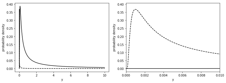
10.2.2 正の値を持つパラメータ

x = np.logspace(-10, 1, 600)
p1 = stats.invgamma.pdf(x, a=0.001, scale=0.001)
p2 = stats.invgamma.pdf(x, a=0.1, scale=0.1)

_, axes = plt.subplots(1, 2, figsize=figaspect(3/8))
for i, ax in enumerate(axes):
    ax.plot(x, p1, c='k', linestyle='dashed')
    ax.plot(x, p2, c='k')
    plt.setp(ax, xlabel='y', ylabel='probability density', xlim=(0, 0.01) if i == 1 else None)
plt.tight_layout()
plt.show()

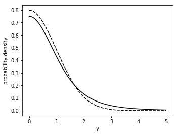
x = np.linspace(0, 5, 101)
p1 = 2*stats.t.pdf(x, df=4)
p2 = 2*stats.norm.pdf(x)

plt.figure(figsize=figaspect(3/4))
ax = plt.axes()
ax.plot(x, p1, c='k')
ax.plot(x, p2, c='k', linestyle='dashed')
plt.setp(ax, xlabel='y', ylabel='probability density')
plt.show()

data = {col: salary2[col] for col in salary2.columns}
data['N'] = salary2.index.size
data['K'] = salary2['KID'].max()

fit1 = pystan.stan('./stan/model8-4b.stan', data=data, seed=1234)
fit2 = pystan.stan('./stan/model8-4d.stan', data=data, seed=1234)

ms1 = fit1.extract()
ms2 = fit2.extract()

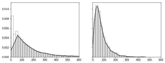
_, axes = plt.subplots(1, 2, figsize=figaspect(3/8), sharex=True, sharey=True)
for ms, ax in zip([ms1, ms2], axes):
    bins = (ms['s_a'].max() - ms['s_a'].min()).astype(int) // 20
    sns.distplot(ms['s_a'], bins=bins, hist_kws=dict(facecolor='w', edgecolor='k'), kde_kws=dict(color='k', shade=True), ax=ax)
    plt.setp(ax, xlim=(0, 600))
plt.show()

N = shogi_player.values.max()
data = dict(
    N=N,
    G=shogi_player.index.size,
    LW=shogi_player
)
fit = pystan.stan('./stan/model10-4.stan', data=data, pars=('mu', 's_mu', 's_pf'), seed=1234)

ms = fit.extract()

d_qua = pd.DataFrame(np.percentile(ms['mu'], (5, 50, 95), axis=0).T, columns=('p05', 'p50', 'p95'))
d_qua['nid'] = np.arange(N) + 1

d_top5 = d_qua.sort_values('p50', ascending=False).head()
d_top5

d_qua = pd.DataFrame(np.percentile(ms['s_pf'], (5, 50, 95), axis=0).T, columns=('p05', 'p50', 'p95'))
d_qua['nid'] = np.arange(N) + 1

d_top3 = d_qua.sort_values('p50', ascending=False).head(3)
d_top3

d_bot3 = d_qua.sort_values('p50').head(3)
d_bot3

10.2.4 分散共分散行列

data = {col: salary2[col] for col in salary2.columns}
data['N'] = salary2.index.size
data['K'] = salary2['KID'].max()
fit = pystan.stan('./stan/model10-5.stan', data=data, seed=1234)

data = {col: salary2[col] for col in salary2.columns}
data['N'] = salary2.index.size
data['K'] = salary2['KID'].max()
fit = pystan.stan('./stan/model10-6.stan', data=data, seed=1234)

data = {col: salary2[col] for col in salary2.columns}
data['N'] = salary2.index.size
data['K'] = salary2['KID'].max()
data['Nu'] = 2
fit = pystan.stan('./stan/model10-7.stan', data=data, seed=1234)