株価予測のスコアが67%を出したので、そこまでの経緯の備忘録です。
今回は精度67%まで出すまでの記録を載せます。
モデルの基本的な説明は前回に掲載しています。
今回のコードはGitHubのkabu_pre2.pyです。
結論
先に結論を述べると、前回のモデルを4日分(day_agoを4)にし、隠れ層を100~170、alphaを0.1~0.5にすると67%を安定して確認できた。
67%自体は、前回のモデルを4日分(day_agoを4)にし、隠れ層を100にするだけでも確認できた。
import numpy as np
import pandas as pd
from sklearn.metrics import confusion_matrix
from sklearn import *
import seaborn as sns
from sklearn.model_selection import *
from sklearn.pipeline import Pipeline
from sklearn.preprocessing import StandardScaler
from sklearn.neural_network import MLPClassifier
from sklearn.model_selection import GridSearchCV
import matplotlib.pyplot as plt
import warnings
import mglearn
import random
from sklearn.metrics import confusion_matrix
from sklearn.model_selection import train_test_split
from datetime import datetime
from sklearn.feature_selection import SelectPercentile
import os
import glob

# 実行上問題ない注意は非表示にする
warnings.filterwarnings('ignore')
# data/kabu1フォルダ内にあるcsvファイルの一覧を取得
files = glob.glob("data/kabu1/*.csv")
# 説明変数となる行列X, 被説明変数となるy2を作成
base = 100
day_ago = 4
num_sihyou = 8
reset =True
# すべてのCSVファイルから得微量作成
for file in files:
    temp = pd.read_csv(file, header=0, encoding='cp932')
    temp = temp[['日付','始値', '高値','安値','終値','5日平均','25日平均','75日平均','出来高']]
    temp= temp.iloc[::-1]#上下反対に
    temp2 = np.array(temp)

    # 前日比を出すためにbase日後からのデータを取得
    temp3 = np.zeros((len(temp2)-base, num_sihyou))
    temp3[0:len(temp3), 0] = temp2[base:len(temp2), 4] / temp2[base-1:len(temp2)-1, 4]
    temp3[0:len(temp3), 1] = temp2[base:len(temp2), 1] / temp2[base:len(temp2), 4]
    temp3[0:len(temp3), 2] = temp2[base:len(temp2), 2] / temp2[base:len(temp2), 4]
    temp3[0:len(temp3), 3] = temp2[base:len(temp2), 3] / temp2[base:len(temp2), 4]
    temp3[0:len(temp3), 4] = temp2[base:len(temp2), 5].astype(np.float) / temp2[base:len(temp2), 4].astype(np.float)
    temp3[0:len(temp3), 5] = temp2[base:len(temp2), 6].astype(np.float) / temp2[base:len(temp2), 4].astype(np.float)
    temp3[0:len(temp3), 6] = temp2[base:len(temp2), 7].astype(np.float) / temp2[base:len(temp2), 4].astype(np.float)
    temp3[0:len(temp3), 7] = temp2[base:len(temp2), 8].astype(np.float) / temp2[base-1:len(temp2)-1, 8].astype(np.float)

    # tempX : 現在の企業のデータ
    tempX = np.zeros((len(temp3), day_ago*num_sihyou))

    # 日にちごとに横向きに(day_ago)分並べる
    # sckit-learnは過去の情報を学習できないので、複数日(day_ago)分を特微量に加える必要がある
    # 注:tempX[0:day_ago]分は欠如データが生まれる
    for s in range(0, num_sihyou):
        for i in range(0, day_ago):
            tempX[i:len(temp3), day_ago*s+i] = temp3[0:len(temp3)-i,s]

    # Xに追加
    # X : すべての企業のデータ
    # tempX[0:day_ago]分は削除
    if reset:
        X = tempX[day_ago:]
        reset = False
    else:
        X = np.concatenate((X, tempX[day_ago:]), axis=0)

# 何日後を値段の差を予測するのか
pre_day = 1
# y : pre_day後の終値/当日終値
y = np.zeros(len(X))
y[0:len(y)-pre_day] = X[pre_day:len(X),0]
X = X[:-pre_day]
y = y[:-pre_day]

up_rate =1.03

# データを一旦分別
X_0 = X[y<=up_rate]
X_1 = X[y>up_rate]
y_0 = y[y<=up_rate]
y_1 = y[y>up_rate]

# X_0をX_1とほぼ同じ数にする
X_drop, X_t, y_drop, y_t = train_test_split(X_0, y_0, test_size=0.09, random_state=0)

# 分別したデータの結合
X_ = np.concatenate((X_1, X_t), axis=0)
y_ = np.concatenate((y_1, y_t))
X_train, X_test, y_train, y_test = train_test_split(X_, y_, random_state=0)

# y_train_,y_test2:翌日の終値/当日の終値がup_rateより上か
y_train2 = np.zeros(len(y_train))
for i in range(0, len(y_train2)):
    if y_train[i] <= up_rate:
        y_train2[i] = 0
    else:
        y_train2[i] = 1

y_test2 = np.zeros(len(y_test))
for i in range(0, len(y_test2)):
    if y_test[i] <= up_rate:
        y_test2[i] = 0
    else:
        y_test2[i] = 1
X_train, X_test, y_train, y_test = train_test_split(X_, y_, random_state=0)
pipe = Pipeline([('scaler', StandardScaler()), ('classifier', MLPClassifier(max_iter=200000, alpha=0.001))])

param_grid = {'classifier__hidden_layer_sizes': [(10,), (100,), (500,)]}

grid = GridSearchCV(pipe, param_grid=param_grid, n_jobs=1, cv=2 ,return_train_score=False, scoring="accuracy")
grid.fit(X_train, y_train)
print(grid.cv_results_['mean_test_score'])
print("Best parameters: ", grid.best_params_)
print("grid best score, ", grid.best_score_)
print("Test set score: {:.2f}".format(grid.score(X_test, y_test)))
conf = confusion_matrix(y_test, grid.predict(X_test))
print(conf)

'''出力結果
[0.6632097  0.67099965]
Best parameters:  {'classifier__hidden_layer_sizes': (100,)}
grid best score,  0.6709996467679266
Test set score: 0.67
over time:  00:17:02
[[23934 11997]
 [11216 23628]]
'''
隠れ層、alphaを調整
param_grid = {'classifier__alpha':[0.0005, 0.001, 0.005, 0.01, 0.05, 0.1 ],
              'classifier__hidden_layer_sizes': [(60, ),(70, ), (80, ),(90, ), (100, ), (110, ), (120, ), (130, ), (140, ), (150, ), (160, ), (170, )]}


print(grid.cv_results_['mean_test_score'])
print("Best parameters: ", grid.best_params_)
print("grid best score, ", grid.best_score_)
print("Test set score: {:.2f}".format(grid.score(X_test, y_test2)))

# ヒートマップで確認
xa = 'classifier__hidden_layer_sizes'
xx = param_grid[xa]
ya = 'classifier__alpha'
yy = param_grid[ya]
plt.figure(figsize=(5,8))
scores = np.array(grid.cv_results_['mean_test_score']).reshape(len(yy), -1)
mglearn.tools.heatmap(scores, xlabel=xa, xticklabels=xx,
                      ylabel=ya, yticklabels=yy, cmap="viridis")
'''
start time:  09:04:52
[0.66983634 0.66970917 0.66917697 0.6675521  0.66820676 0.6684187
 0.66648299 0.66292712 0.66562581 0.66385965 0.66300247 0.66399623
 0.66965736 0.66888496 0.66758978 0.66698222 0.66795243 0.66711409
 0.66445308 0.66298363 0.66240433 0.66574826 0.66748617 0.66630402
 0.67171553 0.67057577 0.66944543 0.6672601  0.66794772 0.66719416
 0.66722242 0.66848463 0.6693842  0.66848463 0.66216884 0.66649241
 0.6700624  0.66927587 0.66985988 0.67064641 0.6652349  0.67026021
 0.6675992  0.67008595 0.66846109 0.66872483 0.66701519 0.66769339
 0.66932768 0.67108913 0.67236077 0.67157424 0.67078771 0.67164488
 0.67100436 0.67317556 0.67175321 0.67185211 0.67232309 0.67072648
 0.67026492 0.67025079 0.67186153 0.67162604 0.67227128 0.67201696
 0.67221947 0.6719416  0.67177205 0.67346756 0.67292123 0.67198399]
Best parameters:  {'classifier__alpha': 0.1, 'classifier__hidden_layer_sizes': (150,)}
grid best score,  0.6734675615212528
Test set score: 0.67
[[24254 11677]
 [11667 23177]]
Test set precision score(再現率): 0.66
over time:  11:48:24
'''
ヒートマップ結果
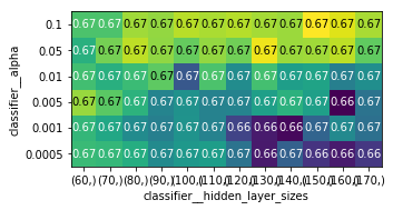
隠れ層を100~170、alphaを0.1~0.5にすると67%を安定して確認できる。
しかし、alphaや隠れ層の10単位で変更しても68以上とならない。
さらなるスコア向上を目指すべく、別パターンを試す。(あまり効果は出なかった。)
day_agoを変えてみる。
day_ago = 2
param_grid = {'classifier__hidden_layer_sizes': [(10,), (100,), (500,)]}
'''出力結果
[0.65889324 0.66886142 0.66844726]
Best parameters:  {'classifier__hidden_layer_sizes': (100,)}
grid best score,  0.668861424349103
Test set score: 0.67
'''
day_ago = 3
param_grid = {'classifier__hidden_layer_sizes': [(10,), (100,), (500,)]}
'''出力結果
[0.6651177  0.66957156 0.6526177 ]
Best parameters:  {'classifier__hidden_layer_sizes': (100,)}
grid best score,  0.6695715630885123
Test set score: 0.67
'''
day_ago = 5
param_grid = {'classifier__hidden_layer_sizes': [(10,), (100,), (500,)]}
'''出力結果
[0.6654904  0.669104   0.66197103]
Best parameters:  {'classifier__hidden_layer_sizes': (100,)}
grid best score,  0.669103998040084
Test set score: 0.67
'''
2-5日程度であれば、隠れ層を100にすると精度66%を確認できた。逆に日数をあまり増やしすぎるとスコアの下落を確認。
スコア向上のヒントを探るべく、一目均衡表,転換線,基準線,先行スパン1,先行スパン2,25日ボリンジャーバンドを追加してみる。(ニューラルネットワークにはこうした加工した得微量はあまり意味を持たないが、25日前の情報も含むため、一応確認。)
一目均衡表,転換線,基準線,先行スパン1,先行スパン2,25日ボリンジャーバンド 追加
day_ago = 3
num_sihyou = 16
# 一目均衡表,転換線,基準線,先行スパン1,先行スパン2,25日ボリンジャーバンド 追加
# 一目均衡表を追加 (9,26, 52)
    para1 =9
    para2 = 26
    para3 = 52
    temp2_2 = np.c_[temp2, np.zeros((len(temp2), 3))]
    p1 = 9
    p2 = 10
    p3 =11

    # 転換線 = (過去(para1)日間の高値 + 安値) ÷ 2
    for i in range(para1, len(temp2)):
        tmp_high =temp2[i-para1+1:i+1,2].astype(np.float)
        tmp_low =temp2[i-para1+1:i+1,3].astype(np.float)
        temp2_2[i, p1] = (np.max(tmp_high) + np.min(tmp_low)) / 2 /temp2[i, 4]

    temp3[0:len(temp3), 8] = temp2_2[base:len(temp2), p1]

    # 基準線 = (過去(para2)日間の高値 + 安値) ÷ 2
    for i in range(para2, len(temp2)):
        tmp_high =temp2[i-para2+1:i+1,2].astype(np.float)
        tmp_low =temp2[i-para2+1:i+1,3].astype(np.float)
        temp2_2[i, p2] = (np.max(tmp_high) + np.min(tmp_low)) / 2 /temp2[i, 4]
    temp3[0:len(temp3), 9] = temp2_2[base:len(temp2), p2]


    # 先行スパン1 = { (転換値+基準値) ÷ 2 }を(para2)日先にずらしたもの
    temp3[0:len(temp3), 10] = (temp2_2[base-para2:len(temp2)-para2, p1] + temp2_2[base-para2:len(temp2)-para2, p2]) /2 /temp2[base:len(temp2), 4]

    # 先行スパン2 = { (過去(para3)日間の高値+安値) ÷ 2 }を(para2)日先にずらしたもの
    for i in range(para3, len(temp2)):
        tmp_high =temp2[i-para3+1:i+1,2].astype(np.float)
        tmp_low =temp2[i-para3+1:i+1,3].astype(np.float)
        temp2_2[i, p3] = (np.max(tmp_high) + np.min(tmp_low)) / 2 /temp2[i, 4]
    temp3[0:len(temp3), 11] = temp2_2[base-para2:len(temp2)-para2, p3]

    # 25日ボリンジャーバンド(±1, 2シグマ)を追加
    parab = 25
    for i in range(base, len(temp2)):
        tmp25 = temp2[i-parab+1:i+1,4].astype(np.float)
        temp3[i-base,12] = np.mean(tmp25) + 1.0* np.std(tmp25)
        temp3[i-base,13] = np.mean(tmp25) - 1.0* np.std(tmp25)
        temp3[i-base,14] = np.mean(tmp25) + 2.0* np.std(tmp25)
        temp3[i-base,15] = np.mean(tmp25) - 2.0* np.std(tmp25)
'''出力結果
[0.66537194 0.66843691 0.6497081 ]
Best parameters:  {'classifier__hidden_layer_sizes': (100,)}
grid best score,  0.668436911487759
Test set score: 0.67
'''
day_ago = 3
num_sihyou = 12
# 一目均衡表,転換線,基準線,先行スパン1,先行スパン2,追加

'''出力結果
[0.66653484 0.6696516  0.64932674]
Best parameters:  {'classifier__hidden_layer_sizes': (100,)}
grid best score,  0.6696516007532957
Test set score: 0.67
'''
得微量が増えたことで、むしろスコアをわずかに落とした。
今まで加えていない曜日情報も試したが、同様の結果となった。
day_ago = 3
num_sihyou = 8
# 曜日情報の追加
ddata = pd.to_datetime(temp['日付'], format='%Y%m%d')
daydata = ddata[base:len(temp2)].dt.dayofweek
daydata_dummies = pd.get_dummies(daydata, columns=['Yobi'])
daydata2 = np.array(daydata_dummies)
tempX = np.concatenate((tempX, daydata2), axis=1)
'''出力結果
[0.66510358 0.66762241 0.6524435 ]
Best parameters:  {'classifier__hidden_layer_sizes': (100,)}
grid best score,  0.6676224105461394
Test set score: 0.67
'''
day_ago = 3
num_sihyou = 16
# 一目均衡表,転換線,基準線,先行スパン1,先行スパン2,25日ボリンジャーバンド, 曜日 追加
'''出力結果
[0.6695951  0.67004237 0.64863936]
Best parameters:  {'classifier__hidden_layer_sizes': (100,)}
grid best score,  0.6700423728813559
Test set score: 0.68
'''
この他にも、day_agoを増やす、上述のパターンから短編量統計を用いて得微量の削減を行ったが、67%より落ちることが多かった。
68%を上回るモデルの改良には、他の方が行っている為替などの情報や、テキストマイニング等を追加してみることだろうか?
現在、同じ日時の紐付け中に起こる欠損データと格闘中。
質問やコメントお待ちしております。