Billboard×Spotifyで「〇〇年代を代表する曲」を決めよう！

はじめに

私は音楽鑑賞が趣味で, 大学ではビルボード研究会というサークルに入っているのですが, 不真面目な部員なのでビルボードチャートをチェックするのは年に数回で, 自分の好きな音楽ばかり聴いています.
「たまにはビルボードを研究しなければ」と思い立ったので, Pythonを使ってデータ解析的な研究をしてみることにしました.

全体としては,
1. Billboard Year-End Hot 100のリストを1950年から2017年まで取得する
2. 1のリストの全曲についてSpotifyが公開しているAudio Featuresを取得する
3. データを観察する
4. 主成分分析で次元削減してプロットする
5. 各曲を年代ごとにグループ分けして, 各グループで重心から最も近いものを調べる
という流れで進めていきます.
アルゴリズムやコードの解説もしながら進めていくので, 結果が気になる人は最後まで飛ばしてください.

データの用意

Billboard Year-End Hot 100

ビルボードは1950年から継続的に, 1年間で最も流行した曲のランキングを作っています.
当初の評価基準はレコードの売上枚数でしたが, その後の視聴形態の変化に合わせてCD売上枚数, ダウンロード数, ストリーミング再生数なども比較的柔軟に加味しているため, その年の流行をよく反映していると考えられます.

なお, 100曲選ばれたのは1959年からで, 1950年から1955年の間は30曲, 1956年から1958年までは50曲のみが選ばれました.

公式サイトはこちらですが, ほとんど遡ることができません.
データベースやAPIのようなものもなさそうなので, 『ウェブスクレイピングで77年分のビルボード年間トップ100を取得してみた. - ただの風邪. 』を参考に, 非公式サイト『Billboard Top 100 Songs of Every Year』から取得しました. 非公式なので正確性は保証できません.
こちらが実行したコードです.

billboard_csv.py

import requests, csv
from bs4 import BeautifulSoup
from time import sleep

for year in range(1945,2018):
    print(year)
    # その年のチャートにアクセスしてランキング部分を取り出す
    url = "http://billboardtop100of.com/" + str(year) + "-2/"
    r = requests.get(url)
    soup = BeautifulSoup(r.content, "html.parser")
    items = soup.find_all("td")
    # ランキングをリストにまとめる
    # カンマはcsvの区切り文字に使うので消去
    chart = [["rank", "artist name", "song title"]]
    for i, item in enumerate(items):
        if i % 3 == 0:
            chart.append([items[i].text,
                          items[i + 1].text.replace(",",""),
                          items[i + 2].text.replace(",","")])
    # CSVファイルに保存
    with open('../billboard_csv/' + str(year) + '.csv', 'w', encoding='utf-8') as f:
        writer = csv.writer(f, lineterminator='\n')
        writer.writerows(chart)
    # サーバに負荷をかけすぎないように, 必ず入れてください
    sleep(5)

失敗した分(確か2013年)や足りない分(2017年)はWikipediaから手動で取りました.
最初からWikipediaからスクレイピングすれば良かったような気もしますが, ページごとに仕様が統一されていなかったり, 更新が頻繁だったりするとコードが使えないという問題があります.
ともあれ, これで計6230曲が集まりました.

Spotify Audio Features

次にこのデータの特徴量をSpotify Web APIを使って取得します.
まずはSpotify for Developersでアカウント登録し, アプリケーションを作ってClient IDとClient Secretを控えてください.
次にAPIを利用するためのライブラリspotipyをインストールします.

$ pip install spotipy

APIを使う前に, 特徴量として利用するAudio Featuresについて説明します.
レファレンスを日本語でまとめてみました.

名前	型	説明
acousticness	float	どれだけアコースティックか. 0.0-1.0
danceability	float	テンポ, リズムの定常性, ビート強度の複合指標. 0.0-1.0
duration_ms	int	トラックの長さ
energy	float	感覚的な音の強さ. 0.0-1.0
instrumentalness	float	ボーカルが少なければ1.0, 多ければ0.0
key	int	キーを整数に直したもの. 例えばCが0
liveness	float	音源に聴衆の音が含まれている度合い. 0.0-1.0
loudness	float	音圧レベル[dB]. -60.0-0.0
mode	int	メジャーなら1, マイナーなら0
speechiness	float	どれだけスピーチに近いか. 0.0-1.0
tempo	float	Beats Per Minute
time_signature	int	拍子. 1小節の中の拍の数
valence	float	ポジティブさ. 0.0-1.0

以上の13特徴量を利用します.
duration_msやloudnessのように定義が明確なものもあれば, acousticnessやvalenceのようにSpotify独自の指標もありますね.
Spotifyはこれらを使ってレコメンドなどを行っているのだと思いますが, 内部のデータを公開してくれるのはありがたいです.

さて, 特徴量取得の流れとしては,
1. ビルボードチャートの曲名とアーティスト名のクエリをSpotifyに送り, 曲のIDを受け取る
2. IDをSpotifyに送り, 曲の特徴量を受け取る
という2段階になります. これをまたCSVファイルにまとめます.
*私はClient IDとClient Secretを.envに保存しました

spotify_csv.py

import  pandas as pd
import re
from tqdm import tqdm
import time
import spotipy
from spotipy.oauth2 import SpotifyClientCredentials

class SpotifyMethods:
    @classmethod
    def __init__(self):
        with open("./.env") as f:
            data = f.readlines()
        client_id = data[0][data[0].find("'")+1:-2]
        client_secret = data[1][data[1].find("'")+1:-2]
        credentials_manager = SpotifyClientCredentials(client_id, client_secret)
        self.sp = spotipy.Spotify(client_credentials_manager=credentials_manager)

    # dataframeに含まれる曲のIDを取得する
    @classmethod
    def getID(self, dataframe):
        ids = []
        for i in range(len(dataframe)):
            query = transform(dataframe.iloc[i]["artist name"]) + " " + transform(dataframe.iloc[i]["song title"])
            results = self.sp.search(q=query, type='track', limit=1)
            if len(results["tracks"]["items"])>0:
                track_id = results['tracks']['items'][0]["id"]
            else:
                track_id = None
            ids.append(track_id)
            time.sleep(1) # 必ず入れる
        return ids

# 曲名とアーティスト名から記号や"feat"以下などを取り除く
def transform(string):
    l = string.lower().replace(".", "").replace("&", "").replace("-", " ").split(" ")
    if "featuring" in l:
        l = l[:l.index("featuring")]
    if "feat" in l:
        l = l[:l.index("feat")]
    return " ".join(l)

def main():
    sm = SpotifyMethods()
    df_all = pd.DataFrame(index=[], columns=['rank', 'artist name', 'song title', 'id', 'year', 'danceability',
       'energy', 'key', 'loudness', 'mode', 'speechiness', 'acousticness',
       'instrumentalness', 'liveness', 'valence', 'tempo', 'type', 'uri',
       'track_href', 'analysis_url', 'duration_ms', 'time_signature',
       'decade'])
    sr_none = pd.Series([None]*len(df_all.columns), index=df_all.columns)

    for year in range(1950,1950):
        df = pd.read_csv("../spotify_csv/"+str(year)+".csv")
        df_all = df_all.append(df, ignore_index=True)

    for year in tqdm(range(1950,2018)):
        df = pd.read_csv("../billboard_csv/"+str(year)+".csv")
        df["year"] = year
        df["decade"] = (df["year"]-1900)//10
        df["id"] = sm.getID(df) # IDを取得
        df = df.dropna() # 欠損値のある行を取り除く
        features = sm.sp.audio_features(df["id"].values) # 特徴量を取得
        for i in range(len(features)):
            if features[i] is None:
                features[i] = sr_none
        keys = features[0].keys()
        for key in keys:
            df[key] = [features[i][key] for i in range(len(features))]
        df = df.dropna() # 欠損値のある行を取り除く
        print(year, len(df))
        df.to_csv("../spotify_csv/"+str(year)+".csv", sep=",", index=False)
        df_all.append(df, ignore_index=True)

    df_all.to_csv("../spotify_csv/all.csv", sep=",", index=False)
    print(len(df_all), "tracks in total")

if __name__ == "__main__":
    main()

クエリを作るところは少し注意が必要です.
例えば, transform関数で全ての記号を削除してしまうと"Ke$ha"が"Keha"となってしまいIDが見つかりません.
また, featuringのアーティストをたくさん入れすぎると, これもIDが見つからない原因になります.
落とし所として, "featuring"以下や".", "&", "-"を消すことにしましたが, もっと良い処理があるかもしれません. 曲名の中の"()"は消すべきだったかもしれません.
欠損値を除いて最終的に特徴量が得られたのは全体で6112曲分(98.1%)でした.
ただし, これも全て意図した曲のIDが取れているとは限りません. 曲名が同じでもカラオケ音源などややこしいものが混ざっている可能性があります(面倒なので確認しませんでした).
結果はこちらで公開しています.

データの可視化

*ここからはJupyter Notebookで分析しました.
必要なライブラリをインポートしてください.

import numpy as np
import  pandas as pd
from matplotlib import pyplot as plt
from sklearn.preprocessing import StandardScaler
from sklearn.decomposition import PCA
from mpl_toolkits.mplot3d import Axes3D

得られたデータのうち, 値が0から1に固定されているものを年ごとに平均してプロットしてみました.

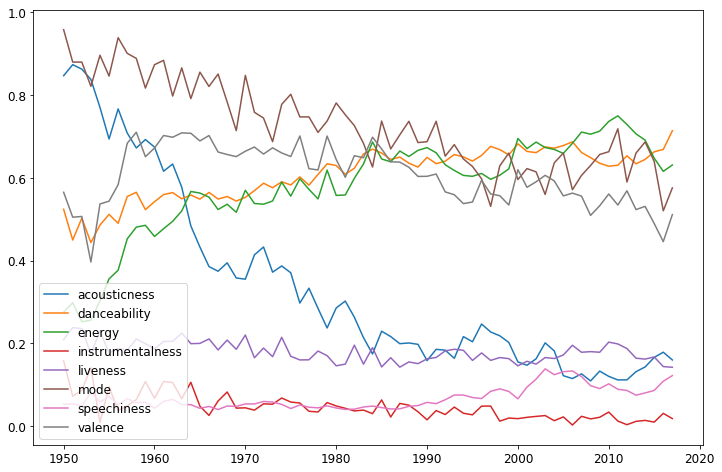
danceabilityとenergyが増加している一方, acousticnessとmodeが減少しています.
danceability, energy, acousticnessに関しては電子楽器の発達やEDMの流行と関係がありそうです.
modeの減少はマイナー調のヒット曲が増えたことを示していますが, この傾向があるとは知りませんでした.
また, よく見るとspeechinessがじわじわと上がっていますが, これはラップの流行によるものでしょう.
*ラップのspeechinessは0.5程度ですが, 他のジャンルの音楽で概ね0.1以下であるのに比べると大きいと言えます

次に, 残りのデータを0から1に収まるように正規化してプロットしてみました.

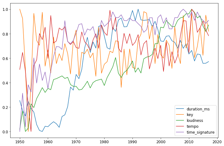
loudnessとtime_signatureが増加しています.
duration_msは1993年頃をピークに減少しています.

主成分分析

主成分分析(promary component analysis; PCA)という手法を使って次元削減を行うと, 13個の特徴量を一目で見ることができます.
今, 各曲は13本の軸を持つ13次元空間上にある点だと考えます.
PCAによる次元削減は, これらの点の分散(広がり)が最も大きくなるような位置から光を当ててその影を見ているというイメージです.
計算方法が気になる方は, このPDFあたりをご覧ください.
第2主成分までを元の軸とともにプロットしたコードと図がこちらです.

def byplot2d(dataframe, arrow_mul=1, text_mul=1.1):
    ss = StandardScaler()
    X = ss.fit_transform(dataframe.drop(["decade"], axis=1).values)
    feature_names = dataframe.drop(["decade"], axis=1).columns

    pca = PCA(n_components=2)
    X = pca.fit_transform(X)
    pc0 = pca.components_[0]
    pc1 = pca.components_[1]

    plt.figure(figsize=(10,10))
    colors = ['#FF00D9', '#FF001A', '#FFA500', '#FFED00', '#00FF75', '#00FFFF', '#6500FF']
    labels = ['50s', '60s', '70s', '80s', '90s', '00s', '10s'] 
    st = 0
    for dec in range(5,12):
        ed = st+len(df_all.loc[df_all["decade"]==dec])
        plt.scatter(X[st:ed,0], X[st:ed,1],
                c=colors[dec-5], marker=".", alpha=0.6, label=labels[dec-5])
        st = ed
    plt.legend(fontsize=15, loc='upper right', frameon=True, facecolor="white")

    print('各次元の寄与率: {0}'.format(pca.explained_variance_ratio_))
    print('累積寄与率: {0}'.format(sum(pca.explained_variance_ratio_)))

    for i in range(pc0.shape[0]):
        plt.arrow(0, 0, 
                  pc0[i]*arrow_mul, pc1[i]*arrow_mul,
                  color='black')
        plt.text(pc0[i]*arrow_mul*text_mul,
                 pc1[i]*arrow_mul*text_mul,
                 feature_names[i],
                 color='black',  fontsize=16)
    plt.show()

byplot2d(df.drop(["artist name", "song title", "rank", "year"], axis=1), arrow_mul=12)

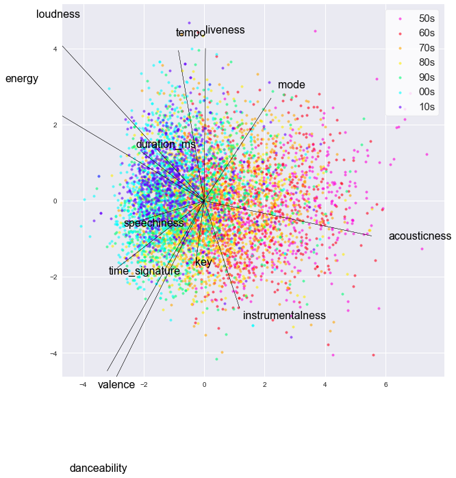
時代が進むにつれて点群がグラフ上を右から左に移動しているのがわかります.
この動きに対応する軸は, acousticness, loudness, energy, duration_msあたりです.

第3主成分までをプロットしたコードと図がこちらです.

def byplot3d(dataframe):
    ss = StandardScaler()
    X = ss.fit_transform(dataframe.drop(["decade"], axis=1).values)

    pca = PCA(n_components=3)
    X = pca.fit_transform(X)

    fig = plt.figure(figsize=(10,8))
    ax = fig.add_subplot(111, projection='3d')
    colors = ['#FF00D9', '#FF001A', '#FFA500', '#FFED00', '#00FF75', '#00FFFF', '#6500FF']
    labels = ['50s', '60s', '70s', '80s', '90s', '00s', '10s'] 
    st = 0
    for dec in range(5,12):
        ed = st+len(df_all.loc[df_all["decade"]==dec])
        ax.scatter(X[st:ed,0], X[st:ed,1], X[st:ed,2],
                c=colors[dec-5], marker=".", alpha=0.6, label=labels[dec-5])
        st = ed
    ax.set_xlim(-3, 3)
    ax.set_ylim(-3, 3)
    ax.set_zlim(-2.5, 2.5)
    plt.legend(fontsize=15, loc='upper left', frameon=True, facecolor="white")
    plt.show()

    print('各次元の寄与率: {0}'.format(pca.explained_variance_ratio_))
    print('累積寄与率: {0}'.format(sum(pca.explained_variance_ratio_)))

byplot3d(df.drop(["artist name", "song title", "rank", "year"], axis=1))

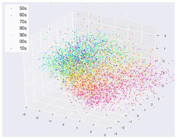
綺麗な図が書けて満足です.

「代表する曲」の検討

各年代グループの重心から近い曲を調べてみましょう.
「近さ」を測る指標としては, 普段から馴染深いユークリッド距離ではなく, 分布の歪みを考慮したマハラノビス距離を使います.
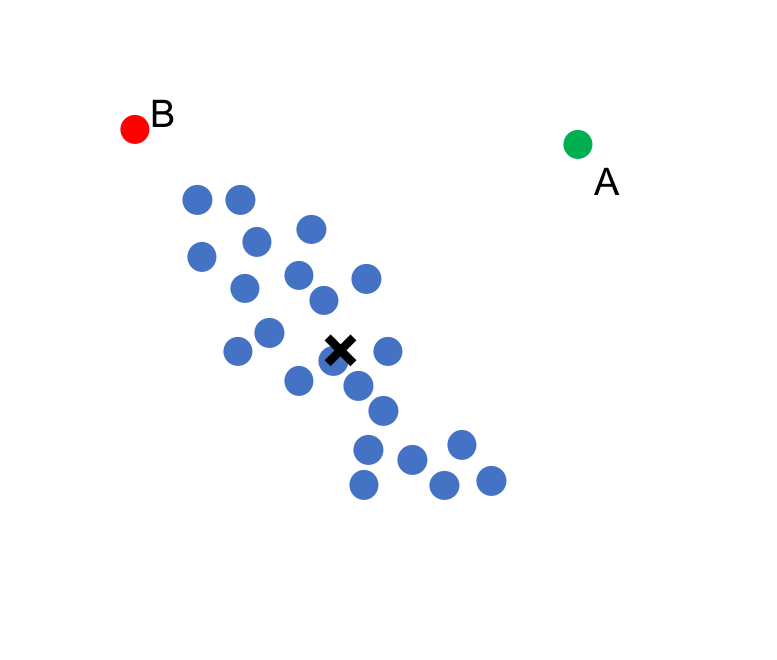
下図の例でいうと, 青い点群の重心から点A, Bまでのユークリッド距離は等しいですが, 点群の分布の形を考えるとBよりも, Aの方が遠くなってほしいですよね. こういう状況ではマハラノビス距離が役に立ちます.

点群の重心のベクトル(列ベクトル)を$\mu$, 点Xのベクトルを$x$とすると, ユークリッド距離は以下のように定義されます.

d_E = \sqrt{(x-\mu)^T(x-\mu)}

一方, マハラノビス距離は, 点群の各次元の分散共分散行列$\Sigma$を用いて次のように定義されます.

d_M = \sqrt{(x-\mu)^T \Sigma^{-1}(x-\mu)}

詳しくは, 『教師なし学習による異常値検知(1): マハラノビス距離 - 未来永劫』あたりがわかりやすいです.

以下の実装では, 複数の曲に対するマハラノビス距離(の二乗)を行列で一気に計算し, 距離の最も短い10曲を出力しています.

st = 0
X = ss.fit_transform(df.drop(["artist name", "song title", "rank", "decade", "year"], axis=1).values)
for dec in range(5,12):
    ed = st+len(df_all.loc[df_all["decade"]==dec])
    Xdec = X[st:ed,:]
    Xdec_mean = np.mean(Xdec, axis=0)
    cov = np.cov(Xdec.T)
    distances = np.diag(np.dot(np.dot(Xdec, np.linalg.inv(cov)), Xdec.T)) # 距離の2乗
    print(distances.shape)
    i_mins = np.argsort(distances)[:10]
    val_mins = distances[i_mins]
    print("\nDecade:", dec)
    for i in range(10):
        song = df.loc[st+i_mins[i],["song title"]].values[0]
        artist = df.loc[st+i_mins[i],["artist name"]].values[0]
        val = round(val_mins[i],2)
        year = df.loc[st+i_mins[i],["year"]].values[0]
        rank = df.loc[st+i_mins[i],["rank"]].values[0]
        print("|", i+1, "|", song, "|", artist, "|", val, "|", year, "|", rank, "|")
    st = ed

結果発表！

1950年代

順位	曲名	アーティスト	距離	年	ランク
1	The Banana Boat Song	Tarriers	6.68	1957	26
2	Poison Ivy	Coasters	10.07	1959	54
3	Lazy Mary	Lou Monte	10.36	1958	80
4	Shake Rattle And Roll	Bill Haley and His Comets	11.95	1954	26
5	Be-bop-a-lula	Gene Vincent	12.67	1956	27
6	At The Hop	Danny and The Juniors	13.02	1958	20
7	Sea Cruise	Frankie Ford	13.12	1959	89
8	Alvin’s Harmonica	David Seville and The Chipmunks	13.36	1959	48
9	Rock-a-Bye Your Baby with a Dixie Melody	Jerry Lewis	13.39	1957	64
10	Witch Doctor	David Seville	13.45	1958	4

Beatles以前はよくわかりません…

1960年代

順位	曲名	アーティスト	距離	年	ランク
1	Hungry	Paul Revere and The Raiders	1.93	1966	97
2	I Got The Feelin’	James Brown and The Famous Flames	3.91	1968	58
3	San Francisco	Scott Mckenzie	4.04	1967	48
4	We Gotta Get Out Of This Place	Animals	4.63	1965	86
5	Polk Salad Annie	Tony Joe White	4.78	1969	77
6	Windy	Association	4.81	1967	4
7	Sunshine Superman	Donovan	4.82	1966	26
8	It’s Now Or Never	Elvis Presley	4.93	1960	7
9	It Hurts To Be In Love	Gene Pitney	4.96	1964	27
10	Mr. Sun Mr. Moon	Paul Revere and The Raiders	5.02	1969	95

60年代らしく、クラシックロックと称されるジャンルの曲が多いです。

1970年代

順位	曲名	アーティスト	距離	年	ランク
1	You’re No Good	Linda Ronstadt	2.7	1975	50
2	Loves Me Like A Rock	Paul Simon	2.76	1973	27
3	Make Me Smile	Chicago	2.88	1970	59
4	Undercover Angel	Alan O’Day	3.35	1977	9
5	Get Down Get Down (Get On The Floor)	Joe Simon	3.39	1975	76
6	How Much I Feel	Ambrosia	3.56	1979	84
7	Dazz	Brick	3.57	1977	41
8	Rock Me Gently	Andy Kim	3.64	1974	29
9	Hot Child In The City	Nick Gilder	3.65	1978	22
10	My Maria	B.W. Stevenson	3.72	1973	64

1980年代

順位	曲名	アーティスト	距離	年	ランク
1	(Keep Feeling) Fascination	Human League	3.75	1983	33
2	Penny Lover	Lionel Richie	4.35	1985	96
3	Ebony And Ivory	Paul McCartney and Stevie Wonder	4.51	1982	4
4	Our House	Madness	4.88	1983	53
5	Open Your Heart	Madonna	4.93	1987	30
6	Express Yourself	Madonna	4.94	1989	55
7	California Girls	David Lee Roth	4.99	1985	88
8	Real Love	Jody Watley	5.28	1989	46
9	867-5309 (Jenny)	Tommy Tutone	5.35	1982	16
10	Coward Of The County	Kenny Rogers	5.48	1980	34

これはしっくりくる結果ですね！

1990年代

順位	曲名	アーティスト	距離	年	ランク
1	Dreamlover	Mariah Carey	2.56	1993	8
2	Place In This World	Michael W. Smith	2.83	1991	77
3	Last Kiss	Pearl Jam	2.84	1999	23
4	Uhh Ahh	Boyz II Men	2.84	1992	84
5	2 Become 1	Spice Girls	2.95	1997	35
6	Fantasy	Mariah Carey	3.13	1995	7
7	Back For Good	Take That	3.17	1995	62
8	Everyday Is A Winding Road	Sheryl Crow	3.48	1997	60
9	Joyride	Roxette	3.55	1991	23
10	It’s Your Love	Tim McGraw and Faith Hill	3.68	1997	40

2000年代

順位	曲名	アーティスト	距離	年	ランク
1	No Shoes No Shirt No Problems	Kenny Chesney	2.85	2003	91
2	The Good Stuff	Kenny Chesney	3.17	2002	82
3	Here (In Your Arms)	Hellogoodbye	4.01	2007	81
4	Living and Living Well	George Strait	4.18	2002	93
5	Fallin’ For You	Colbie Caillat	4.22	2009	68
6	TRUE	Ryan Cabrera	4.29	2005	90
7	You’ll Think of Me	Keith Urban	4.31	2004	93
8	Let Me Love You	Mario	4.38	2005	3
9	Beer for my Horses	Toby Keith Duet With Willie Nelson	4.74	2003	75
10	I Don’t Want to Be	Gavin DeGraw	4.83	2005	58

Kenny Chesneyというカントリー歌手が１位と2位になりました.
2000年代はカントリーが流行っていたのでしょうか…？

2010年代

順位	曲名	アーティスト	距離	年	ランク
1	Good Life	OneRepublic	4.11	2011	25
2	Knee Deep	Zac Brown Band feat. Jimmy Buffett	4.33	2011	80
3	Wildest Dreams	Taylor Swift	4.73	2015	57
4	Burnin’ It Down	Jason Aldean	5.01	2014	63
5	Gone Gone Gone	Phillip Phillips	5.09	2013	61
6	Pompeii	Bastille	5.21	2014	12
7	22	Taylor Swift	5.26	2013	71
8	Team	Lorde	5.34	2014	18
9	Firework	Katy Perry	5.58	2011	3
10	You And Tequila	Kenny Chesney feat. Grace Potter	5.71	2011	98

Taylor vs Katyの戦い, ここではTaylor勝利です.

「〇〇年代を代表しない曲」

ちなみに, 先ほどのコードでi_mins = np.argsort(distances)[:10]のインデックスの部分を[-10:]とすれば, 重心から最も遠い10曲を選べます.
結果を1曲ずつだけ紹介します.

年代	曲名	アーティスト	距離	年	ランク
50	St. George And The Dragonet	Stan Freberg	186.7	1953	15
60	Delilah	Tom Jones	83.7	1968	66
70	Tubular Bells	Mike Oldfield	259.65	1974	79
80	A Love Bizarre	Sheila E.	95.87	1986	83
90	Now And Forever	Richard Marx	170.21	1994	25
00	Wanna Get To Know You	G-Unit feat. Joe	189.21	2004	86
10	Imma Be	Black Eyed Peas	287.29	2010	20

全体的によくわからない結果です.
Tubular Bellsは, 収録時間が26分とduration_msが外れ値的に大きいです.

プレイリスト

知らない曲も多かったので, プレイリストにまとめてみました！
Songs That Defined X0's | Spotify
Songs That DID NOT Define X0's | Spotify

感想

やる前からわかってはいましたが, 結果の解釈が難しいですね…
「わかるような, わからないような」というのが正直な感想です.
ただ, 年間の売り上げや順位のような「人による評価」を利用しなかったため, 音楽メディアが選ぶ「〇〇年代を代表する曲」とは全く異なる結果が出ておもしろかったです.