PCRより感度が高い？深層学習を用いて胸部レントゲン画像からCOVID-19を検出する

目的

初投稿のためキャッチーなタイトルをつけたが、本記事の目的は、書籍「作りながら学ぶ　Pytorchによる発展ディープラーニング」を元にVGG19を用いたFine tuningを学ぶ過程を記録することである。

使用するデータセットは、COVID-19 Radiography Databaseで公開されている胸部レントゲン写真を用いる。

0. 背景

VGG19は、「ImageNet」と呼ばれる大規模画像データセットで学習された畳み込みニューラルネットワークモデルVGG-16の拡張版である。畳み込み層、プーリング層、全結合層からなる非常にシンプルなモデルであり、初学者でもいじれる事が期待される。

転移学習とは、ある領域で学習したこと(学習済みモデル)を別の領域に利用する手法である。狭義には、最終の出力層のみを目的のデータセット用に付け替えて学習させることを指す。入力層に近い層のパラメタも更新する場合はFine tuningと呼ばれる。

なお、本データセットはarxivに投稿された論文Muhammad E. H. Chowdhury, et al., Can AI help in screening Viral and COVID‐19 pneumonia?の筆者らが整備したものである。
また本モデルは学習・研究用途のため構築したものであり、診断目的には使用できない。

200421追記 注意

今回使用したデータセットは、normalおよびviral pneumoniaのデータはkaggleにある同一のデータセットから取ってきている一方、COVID-19のデータセットは複数のウェブサイト、論文からかき集めています。また、よく見るとCOVID-19のデータには重複がある、側面からの写真があるなど、そのまま使用するにはデータの質自体に問題があることがわかりました。
ですので、今回思いの他高い性能が出たのは、単にデータセットの質の違いを単純に反映している可能性もあります。

1. google colabの設定

google colabを開いて新規ノートブックを作成し、googleドライブをマウントする。

from google.colab import drive
drive.mount('/content/drive')

ランタイムのタイプをGPUに変更する。

2. データのダウンロード

COVID-19 Radiography Databaseからデータをダウンロードし（kaggleの登録が必要）、google drive上の任意の場所へアップロードする。
データは、Normal 1341枚、COVID-19 219枚、Viral Pneumonia 1345枚
中身をよく見ると、側面から撮られた画像もあるため取り除いた方が良い。

3. パッケージインポート

# パッケージのimport, 整理できていない
import glob
import os.path as osp
import os
import random
import numpy as np
import pandas as pd
import sklearn
import json
import time
import PIL
from PIL import Image
from tqdm import tqdm
import matplotlib.pyplot as plt
%matplotlib inline

import torch
import torchvision
from torch.autograd import Variable
import torch.nn as nn
import torch.nn.functional as F
import torch.optim as optim
from torchvision import models, transforms
from torch.utils.data import DataLoader, TensorDataset
from sklearn.model_selection import train_test_split

# PyTorchのバージョン確認
print("PyTorch Version: ",torch.__version__)
print("Torchvision Version: ",torchvision.__version__)
print("Pillow Version: ",PIL.__version__)

実行結果：

PyTorch Version:  1.4.0
Torchvision Version:  0.5.0
Pillow Version:  7.0.0

GPUが使えるかを確認

device = torch.device("cuda:0" if torch.cuda.is_available() else "cpu")
print("使用デバイス：", device)

実行結果：

使用デバイス： cuda:0

3. 画像データセットの作成

はじめに、画像の前処理クラスImageTransformを作成する。

訓練時と推論時で処理が異なるように書く。

今回は使用しないが、grad-cam実装時に役立つようresizeのみの挙動も設定しておく。

class ImageTransform():
    """
    画像の前処理クラス。訓練時、検証時・推論時で異なる動作をする。
    画像のサイズをリサイズし、色を標準化する。
    訓練時はRandomResizedCropに加え, 
    新たにRandomRotationの操作を加えたデータオーギュメンテーションを行う。
    参考書に書かれたRandomHorizontalFlipは臓器左右反転を考慮しなくて良いと判断し削除した。

    Attributes
    ----------
    resize : int
        リサイズ先の画像の大きさ。
    mean : (R, G, B)
        各色チャネルの平均値。
    std : (R, G, B)
        各色チャネルの標準偏差。
    """

    def __init__(self, resize, mean, std):
        self.data_transform = {
            'train': transforms.Compose([
                transforms.RandomResizedCrop(
                    resize, scale=(0.8, 1.0)),  # あまり小さくなりすぎないように
                #transforms.RandomHorizontalFlip(),  # 反転
                transforms.RandomRotation(degrees=(3, -3)), # -3~3度回転
                transforms.ToTensor(),  # テンソルに変換
                transforms.Normalize(mean, std)  # 標準化
            ]),
            'val': transforms.Compose([
                transforms.Resize(resize),  # リサイズ
                transforms.CenterCrop(resize),  # 画像中央をresize×resizeで切り取り
                transforms.ToTensor(),  # テンソルに変換
                transforms.Normalize(mean, std)  # 標準化
            ]),
            'resize': transforms.Compose([
                transforms.Resize(resize),  # リサイズ
                transforms.CenterCrop(resize),  # 画像中央をresize×resizeで切り取り
                transforms.ToTensor(),  # テンソルに変換
            ])
        }

    def __call__(self, img, phase='train'):
        """
        Parameters
        ----------
        phase : 'train' or 'val' or 'resize'
            前処理のモードを指定。
        """
        return self.data_transform[phase](img)

訓練時の画像前処理の動作を確認する

# 1. 画像読み込み
image_file_path ='/content/drive/My Drive/Colab Notebooks/COVID-19 Radiography Database/NORMAL/NORMAL (1).png'
img = Image.open(image_file_path).convert('RGB')

# 2. 元の画像の表示
plt.imshow(img)
plt.show(img)
print('元画像')

# 3. 画像の前処理と処理済み画像の表示 VGG16の訓練データに揃える
size = 224 #VGG16だと224
mean = (0.485, 0.456, 0.406)
std = (0.229, 0.224, 0.225)

transform = ImageTransform(size, mean, std)
img_transformed = transform(img, phase="train")  # torch.Size([3, 224, 224])

# (色、高さ、幅)を (高さ、幅、色)に変換し、0-1に値を制限して表示
img_transformed = img_transformed.numpy().transpose((1, 2, 0))
img_transformed = np.clip(img_transformed, 0, 1)
plt.imshow(img_transformed)
plt.show()
print('学習画像')

実行結果：

元画像

学習用画像

次に、データリストのパスを格納するリストを用意する

def make_datapath_list(phase="NORMAL", rootpath = "/content/drive/My Drive/Colab Notebooks/COVID-19 Radiography Database/"):
    """
    データのパスを格納したリストを作成する。
    pytorchのtutorialとは異なるディレクトリの構造なので、書き換え
    Parameters
    ----------
    phase : 'Type'
        各画像

    Returns
    -------
    path_list : list
        データへのパスを格納したリスト
    """

    target_path = osp.join(rootpath+phase+'/*.png')
    print(target_path)

    path_list = []  # ここに格納する

    # globを利用してサブディレクトリまでファイルパスを取得する
    for path in glob.glob(target_path):
        path_list.append(path)

    return path_list

# 実行
rootpath = "/content/drive/My Drive/Colab Notebooks/COVID-19 Radiography Database/"
COVID_list = make_datapath_list(phase="COVID-19", rootpath = rootpath)
NORMAL_list = make_datapath_list(phase="NORMAL", rootpath = rootpath)
Pneumonia_list = make_datapath_list(phase="Viral Pneumonia", rootpath = rootpath)

# 学習、検証、テストを6, 2, 2で分ける。
C_tv, C_test = train_test_split(COVID_list, test_size=0.2)
N_tv, N_test = train_test_split(NORMAL_list, test_size=0.2)
P_tv, P_test = train_test_split(Pneumonia_list, test_size=0.2)

C_train, C_valid = train_test_split(C_tv, test_size=0.25)
N_train, N_valid = train_test_split(N_tv, test_size=0.25)
P_train, P_valid = train_test_split(P_tv, test_size=0.25)

train_list = C_train + N_train + P_train
val_list = C_valid + N_valid + P_valid
test_list = C_test + N_test + P_test

print('train :', len(train_list), 'samples, valid :', len(val_list), 'samples, test :', len(test_list), 'samples')

#各リスト書き出し
f = open('/content/drive/My Drive/Colab Notebooks/COVID-19 Radiography Database/train_list.txt', 'w')
for x in train_list:
    f.write(str(x) + "\n")
f.close()
f = open('/content/drive/My Drive/Colab Notebooks/COVID-19 Radiography Database/val_list.txt', 'w')
for x in val_list:
    f.write(str(x) + "\n")
f.close()
f = open('/content/drive/My Drive/Colab Notebooks/COVID-19 Radiography Database/test_list.txt', 'w')
for x in test_list:
    f.write(str(x) + "\n")
f.close()

実行結果

/content/drive/My Drive/Colab Notebooks/COVID-19 Radiography Database/COVID-19/*.png
/content/drive/My Drive/Colab Notebooks/COVID-19 Radiography Database/NORMAL/*.png
/content/drive/My Drive/Colab Notebooks/COVID-19 Radiography Database/Viral Pneumonia/*.png
train : 1742 samples, valid : 581 samples, test : 582 samples

続いて、ファイルパスリストからデータセットを作成する

class HymenopteraDataset(torch.utils.data.Dataset):
    """
    X線画像のDatasetクラス。PyTorchのDatasetクラスを継承。

    Attributes
    ----------
    file_list : リスト
        画像のパスを格納したリスト
    transform : object
        前処理クラスのインスタンス
    phase : 'train' or 'test' or 'resize'
        学習か訓練かを設定する。
    """

    def __init__(self, file_list, transform=None, phase='train'):
        self.file_list = file_list  # ファイルパスのリスト
        self.transform = transform  # 前処理クラスのインスタンス
        self.phase = phase  # train or valの指定

    def __len__(self):
        '''画像の枚数を返す'''
        return len(self.file_list)

    def __getitem__(self, index):
        '''
        前処理をした画像のTensor形式のデータとラベルを取得
        '''
        # index番目の画像をロード
        img_path = self.file_list[index]
        img = Image.open(img_path).convert('RGB') #RGBに変換

        # 画像の前処理を実施
        img_transformed = self.transform(
            img, self.phase)  # torch.Size([3, 224, 224])

        # 画像のラベルをファイル名から抜き出す 下層から２番目のディレクトリ名の頭文字で判断
        label = img_path[len(rootpath)] #rootpathの次の文字で判断

        # ラベルを数値に変更する
        if label == "N":
            label = 0 #Normal
        elif label == "C":
            label = 1 #COVID
        elif label == "V":
            label = 2 #Viral Pneumonia

        return img_transformed, label

# 実行
train_dataset = HymenopteraDataset(
    file_list=train_list, transform=ImageTransform(size, mean, std), phase='train')

val_dataset = HymenopteraDataset(
    file_list=val_list, transform=ImageTransform(size, mean, std), phase='val')

test_dataset = HymenopteraDataset(
    file_list=test_list, transform=ImageTransform(size, mean, std), phase='val')

4. DataLoaderを作成

# ミニバッチのサイズを指定
batch_size = 32

# DataLoaderを作成
train_dataloader = torch.utils.data.DataLoader(
    train_dataset, batch_size=batch_size, shuffle=True)

val_dataloader = torch.utils.data.DataLoader(
    val_dataset, batch_size=batch_size, shuffle=False)

test_dataloader = torch.utils.data.DataLoader(
    test_dataset, batch_size=batch_size, shuffle=False)

# 辞書型変数にまとめる
dataloaders_dict = {"train": train_dataloader,
                    "val": val_dataloader,
                    "test": test_dataloader}

5. ネットワークモデルのロード

1.5章に倣って編集

#学習済みのモデルをロード
use_pretrained = True #学習済みのパラメタを使用
net = models.vgg19(pretrained = use_pretrained)

ネットワーク構造を確認

net

VGG(
  (features): Sequential(
    (0): Conv2d(3, 64, kernel_size=(3, 3), stride=(1, 1), padding=(1, 1))
    (1): ReLU(inplace=True)
    (2): Conv2d(64, 64, kernel_size=(3, 3), stride=(1, 1), padding=(1, 1))
    (3): ReLU(inplace=True)
    (4): MaxPool2d(kernel_size=2, stride=2, padding=0, dilation=1, ceil_mode=False)
    (5): Conv2d(64, 128, kernel_size=(3, 3), stride=(1, 1), padding=(1, 1))
    (6): ReLU(inplace=True)
    (7): Conv2d(128, 128, kernel_size=(3, 3), stride=(1, 1), padding=(1, 1))
    (8): ReLU(inplace=True)
    (9): MaxPool2d(kernel_size=2, stride=2, padding=0, dilation=1, ceil_mode=False)
    (10): Conv2d(128, 256, kernel_size=(3, 3), stride=(1, 1), padding=(1, 1))
    (11): ReLU(inplace=True)
    (12): Conv2d(256, 256, kernel_size=(3, 3), stride=(1, 1), padding=(1, 1))
    (13): ReLU(inplace=True)
    (14): Conv2d(256, 256, kernel_size=(3, 3), stride=(1, 1), padding=(1, 1))
    (15): ReLU(inplace=True)
    (16): Conv2d(256, 256, kernel_size=(3, 3), stride=(1, 1), padding=(1, 1))
    (17): ReLU(inplace=True)
    (18): MaxPool2d(kernel_size=2, stride=2, padding=0, dilation=1, ceil_mode=False)
    (19): Conv2d(256, 512, kernel_size=(3, 3), stride=(1, 1), padding=(1, 1))
    (20): ReLU(inplace=True)
    (21): Conv2d(512, 512, kernel_size=(3, 3), stride=(1, 1), padding=(1, 1))
    (22): ReLU(inplace=True)
    (23): Conv2d(512, 512, kernel_size=(3, 3), stride=(1, 1), padding=(1, 1))
    (24): ReLU(inplace=True)
    (25): Conv2d(512, 512, kernel_size=(3, 3), stride=(1, 1), padding=(1, 1))
    (26): ReLU(inplace=True)
    (27): MaxPool2d(kernel_size=2, stride=2, padding=0, dilation=1, ceil_mode=False)
    (28): Conv2d(512, 512, kernel_size=(3, 3), stride=(1, 1), padding=(1, 1))
    (29): ReLU(inplace=True)
    (30): Conv2d(512, 512, kernel_size=(3, 3), stride=(1, 1), padding=(1, 1))
    (31): ReLU(inplace=True)
    (32): Conv2d(512, 512, kernel_size=(3, 3), stride=(1, 1), padding=(1, 1))
    (33): ReLU(inplace=True)
    (34): Conv2d(512, 512, kernel_size=(3, 3), stride=(1, 1), padding=(1, 1))
    (35): ReLU(inplace=True)
    (36): MaxPool2d(kernel_size=2, stride=2, padding=0, dilation=1, ceil_mode=False)
  )
  (avgpool): AdaptiveAvgPool2d(output_size=(7, 7))
  (classifier): Sequential(
    (0): Linear(in_features=25088, out_features=4096, bias=True)
    (1): ReLU(inplace=True)
    (2): Dropout(p=0.5, inplace=False)
    (3): Linear(in_features=4096, out_features=4096, bias=True)
    (4): ReLU(inplace=True)
    (5): Dropout(p=0.5, inplace=False)
    (6): Linear(in_features=4096, out_features=1000, bias=True)
  )
)

#VGG19の最後の出力ユニットの変更
net.classifier[6] = nn.Linear(in_features=4096, out_features=3)
#訓練モードに設定
net.train()

6. 損失関数の定義および最適化手法の設定

# 損失関数の設定
criterion = nn.CrossEntropyLoss()

# ファインチューニングで学習させるパラメータを、変数params_to_updateの1～3に格納する

params_to_update_1 = []
params_to_update_2 = []
params_to_update_3 = []

# 学習させる層のパラメータ名を指定
update_param_names_1 = ["features"]
update_param_names_2 = ["classifier.0.weight",
                        "classifier.0.bias", "classifier.3.weight", "classifier.3.bias"]
update_param_names_3 = ["classifier.6.weight", "classifier.6.bias"]

# パラメータごとに各リストに格納する
for name, param in net.named_parameters():
    if update_param_names_1[0] in name:
        param.requires_grad = True
        params_to_update_1.append(param)
        print("params_to_update_1に格納：", name)

    elif name in update_param_names_2:
        param.requires_grad = True
        params_to_update_2.append(param)
        print("params_to_update_2に格納：", name)

    elif name in update_param_names_3:
        param.requires_grad = True
        params_to_update_3.append(param)
        print("params_to_update_3に格納：", name)

    else:
        param.requires_grad = False
        print("勾配計算なし。学習しない：", name)

# optim.SGDからoptim.Adamに変更してみる
optimizer = optim.Adam([
    {'params': params_to_update_1, 'lr': 1e-4},
    {'params': params_to_update_2, 'lr': 5e-4},
    {'params': params_to_update_3, 'lr': 1e-3}
])

params_to_update_1に格納： features.0.weight
params_to_update_1に格納： features.0.bias
params_to_update_1に格納： features.2.weight
params_to_update_1に格納： features.2.bias
params_to_update_1に格納： features.5.weight
params_to_update_1に格納： features.5.bias
params_to_update_1に格納： features.7.weight
params_to_update_1に格納： features.7.bias
params_to_update_1に格納： features.10.weight
params_to_update_1に格納： features.10.bias
params_to_update_1に格納： features.12.weight
params_to_update_1に格納： features.12.bias
params_to_update_1に格納： features.14.weight
params_to_update_1に格納： features.14.bias
params_to_update_1に格納： features.16.weight
params_to_update_1に格納： features.16.bias
params_to_update_1に格納： features.19.weight
params_to_update_1に格納： features.19.bias
params_to_update_1に格納： features.21.weight
params_to_update_1に格納： features.21.bias
params_to_update_1に格納： features.23.weight
params_to_update_1に格納： features.23.bias
params_to_update_1に格納： features.25.weight
params_to_update_1に格納： features.25.bias
params_to_update_1に格納： features.28.weight
params_to_update_1に格納： features.28.bias
params_to_update_1に格納： features.30.weight
params_to_update_1に格納： features.30.bias
params_to_update_1に格納： features.32.weight
params_to_update_1に格納： features.32.bias
params_to_update_1に格納： features.34.weight
params_to_update_1に格納： features.34.bias
params_to_update_2に格納： classifier.0.weight
params_to_update_2に格納： classifier.0.bias
params_to_update_2に格納： classifier.3.weight
params_to_update_2に格納： classifier.3.bias
params_to_update_3に格納： classifier.6.weight
params_to_update_3に格納： classifier.6.bias

7. 学習・検証を実施

# モデルを学習させる関数を作成
def train_model(net, dataloaders_dict, criterion, optimizer, num_epochs):

    # 初期設定
    # GPUが使えるかを確認
    device = torch.device("cuda:0" if torch.cuda.is_available() else "cpu")
    print("使用デバイス：", device)
    net.to(device)

    # ネットワークがある程度固定であれば、高速化させる
    torch.backends.cudnn.benchmark = True

    # イテレーションカウンタをセット
    iteration = 1
    epoch_train_loss = 0.0  # epochの損失和
    epoch_val_loss = 0.0  # epochの損失和
    logs = []

    # epochのループ
    for epoch in range(num_epochs):

        # 開始時刻を保存
        t_epoch_start = time.time()
        t_iter_start = time.time()

        epoch_train_acc = 0.0  # epochの正解数
        epoch_val_acc = 0.0  # epochの正解数
        epoch_train_corrects = 0
        epoch_val_corrects = 0

        print('-------------')
        print('Epoch {}/{}'.format(epoch+1, num_epochs))
        print('-------------')

        # epochごとの学習と検証のループ
        for phase in ['train', 'val']:
            if phase == 'train':
                net.train()  # モデルを訓練モードに
                print('（train）')
            else:
                if((epoch+1) % 5 == 0):
                    net.eval()   # モデルを検証モードに
                    print('-------------')
                    print('（val）')
                else:
                    # 検証は5回に1回だけ行う
                    continue                

            # データローダーからミニバッチを取り出すループ
            for inputs, labels in tqdm(dataloaders_dict[phase], position=0, leave=True):

                # GPUが使えるならGPUにデータを送る
                inputs = inputs.to(device)
                labels = labels.to(device)

                # optimizerを初期化
                optimizer.zero_grad()

                # 順伝搬（forward）計算
                with torch.set_grad_enabled(phase == 'train'):
                    outputs = net(inputs)
                    loss = criterion(outputs, labels)  # 損失を計算
                    _, preds = torch.max(outputs, 1)  # ラベルを予測

                    # 訓練時はバックプロパゲーション
                    if phase == 'train':
                        loss.backward() # 勾配の計算
                        optimizer.step() # パラメータ更新
                        # 正解数の合計
                        epoch_train_corrects += torch.sum(preds == labels.data).item()

                        epoch_train_loss += loss.item() * inputs.size(0)
                        iteration += 1

                    # 検証時
                    else:
                        epoch_val_loss += loss.item() * inputs.size(0)
                        epoch_val_corrects += torch.sum(preds == labels.data).item()

        # epochのphaseごとのloss
        t_epoch_finish = time.time()
        print('-------------')
        print('epoch {} || Epoch_TRAIN_Loss:{:.4f} || Epoch_VAL_Loss:{:.4f}'.format(
            epoch+1, epoch_train_loss, epoch_val_loss))

        # epochごとの正解率を表示
        epoch_train_corrects
        epoch_train_acc = epoch_train_corrects / len(dataloaders_dict['train'].dataset)
        epoch_val_acc = epoch_val_corrects / len(dataloaders_dict['val'].dataset)

        print('epoch {} || Epoch_train_accuracy:{:.3f} || Epoch_val_accuracy:{:.3f}'.format(
                epoch+1, epoch_train_acc, epoch_val_acc))

        print('timer:  {:.4f} sec.'.format(t_epoch_finish - t_epoch_start))
        t_epoch_start = time.time()
        print('-------------')

        # ログを保存
        log_epoch = {'epoch': epoch+1,
                     'train_loss': epoch_train_loss,
                     'val_loss': epoch_val_loss,
                     'train_accuracy': epoch_train_acc,
                     'val_accuracy': epoch_val_acc,
                     'epoch_train_corrects': epoch_train_corrects,
                     'epoch_val_corrects': epoch_val_corrects}
        logs.append(log_epoch)
        df = pd.DataFrame(logs)
        df.to_csv("/content/drive/My Drive/Colab Notebooks/COVID-19 Radiography Database/log_output.csv")

        epoch_train_loss = 0.0  # epochの損失和
        epoch_val_loss = 0.0  # epochの損失和
        epoch_train_corrects = 0
        epoch_val_corrects = 0
        #iteration = 1

        # 5回に1回、ネットワークを保存する
        if ((epoch+1) % 5 == 0):
            torch.save(net.state_dict(), '/content/drive/My Drive/Colab Notebooks/COVID-19 Radiography Database/weights_' +
                       str(epoch+1) + '.pth')

# 学習・検証を実行する
num_epochs=30
train_model(net, dataloaders_dict, criterion, optimizer, num_epochs=num_epochs)

実行時間は1epochあたり１分程度であったが不安定。計算機の割り当てられ具合で変動する。

8. 学習、検証結果のloss, accuracyのplot

#lossおよびaccuracyのplot
df = pd.read_csv('/content/drive/My Drive/Colab Notebooks/COVID-19 Radiography Database/log_output.csv')
df.replace([0, 0.0], np.nan, inplace=True)
ax = df.plot.scatter(x='epoch', y='val_loss', c='orange')
df.plot.line(x='epoch', y='train_loss', title='Loss', ax = ax)
axs = df.plot.scatter(x='epoch', y='val_accuracy', c='orange')
df.plot.line(x='epoch', y='train_accuracy', title='Accuracy', ax = axs)

<matplotlib.axes._subplots.AxesSubplot at 0x7fd1e75af940>

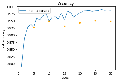
trainに比べてvalのaccracyが改善していない場合、overfittingを考慮する。
もっと学習を回さないと判断が難しいが、10 epoch以降はオーバーフィット気味だと判断できる。

9. test dataのaccuracy

# モデルの呼び出し セッション切れになった場合はネットワーク構造の読み込みから行う。
# net = models.vgg19(pretrained = False)
# net.classifier[6] = nn.Linear(in_features=4096, out_features=3)
# PyTorchのネットワークパラメータのロード
load_path = '/content/drive/My Drive/Colab Notebooks/COVID-19 Radiography Database/'
load_eppochs = 'weights_10.pth'
load_weights = torch.load(load_path + load_eppochs)
net.load_state_dict(load_weights)

#推論モード
net.eval()
net.to(device)
corrects = 0
loss = 0
ANS = []
PRED = []
for inputs, labels in tqdm(dataloaders_dict['test'], position=0, leave=True):
    # GPUが使えるならGPUにデータを送る
    inputs = inputs.to(device)
    labels = labels.to(device)

    outputs = net(inputs)
    loss = criterion(outputs, labels)  # 損失を計算
    _, preds = torch.max(outputs, 1)  # ラベルを予測

    corrects += torch.sum(preds == labels.data).item()
    PRED.extend(preds.tolist())
    ANS.extend(labels.data.tolist())

# epochごとの正解率を表示
accuracy = corrects / len(dataloaders_dict['test'].dataset)
print('test_acc: {:.4f}'.format(accuracy))

test_acc: 0.9570

95.7%正答できるモデルが作成された。

10. 混同行列の表示

## confusion matrix from https://deeplizard.com/learn/video/0LhiS6yu2qQ
stacked = torch.stack(
    (
        torch.LongTensor(ANS), torch.LongTensor(PRED)
    )
    ,dim=1
)
print(stacked.shape)
#matrix雛形
cmt = torch.zeros(3, 3, dtype=torch.int64)
for p in stacked:
    tl, pl = p.tolist()
    cmt[tl, pl] = cmt[tl, pl] + 1
df = pd.DataFrame(cmt.tolist())
names = [
    'Normal'
    ,'COVID-19'
    ,'Viral Pneumonia'
]
df.columns = names
df.index = names
df = df.add_suffix('_pred')
print(df)
df.to_csv(load_path + 'Confusion_matrix.csv')

torch.Size([582, 2])
                 Normal_pred  COVID-19_pred  Viral Pneumonia_pred
Normal                   268              1                     0
COVID-19                   0             42                     2
Viral Pneumonia           22              0                   247

confusion.matrix関数の作成

import itertools
def plot_conf_matrix(cm, classes, normalize=False, title='Confusion matrix', cmap=plt.cm.Blues):
    if normalize:
        cm = cm.astype('float') / cm.sum(axis=1)[:, np.newaxis]
        print("Normalized confusion matrix")
    else:
        print('Confusion matrix, without normalization')

    print(cm)
    plt.imshow(cm, interpolation='nearest', cmap=cmap)
    plt.title(title)
    plt.colorbar()
    tick_marks = np.arange(len(classes))
    plt.xticks(tick_marks, classes, rotation=45)
    plt.yticks(tick_marks, classes)

    fmt = '.2f' if normalize else 'd'
    thresh = cm.max() / 2.
    for i, j in itertools.product(range(cm.shape[0]), range(cm.shape[1])):
        plt.text(j, i, format(cm[i, j], fmt), horizontalalignment="center", color="white" if cm[i, j] > thresh else "black")

    plt.tight_layout()
    plt.ylabel('True label')
    plt.xlabel('Predicted label')

names = (
    'Normal'
    ,'COVID-19'
    ,'Viral Pneumonia'
)
plt.figure(figsize=(4,4))
plot_conf_matrix(cmt, names)
plt.savefig(load_path + 'CM.pdf')

Confusion matrix, without normalization
tensor([[268,   1,   0],
        [  0,  42,   2],
        [ 22,   0, 247]])

11. Precision, recallを計算

# precision recall 
# https://scikitlearn.org/stable/modules/generated/sklearn.metrics.classification_report.html
rep = sklearn.metrics.classification_report(
    ANS, PRED, labels=None, target_names=names,
    sample_weight=None, digits=3, output_dict=True)

report_df = pd.DataFrame(rep)
# index=Falseにするとラベル名が消えてしまうので注意
report_df.to_csv(load_path + "report.csv")
report_df

	Normal	COVID-19	Viral Pneumonia	accuracy	macro avg	weighted avg
precision	0.924138	0.976744	0.991968	0.957045	0.964283	0.959466
recall	0.996283	0.954545	0.918216	0.957045	0.956348	0.957045
f1-score	0.958855	0.965517	0.953668	0.957045	0.959347	0.956961
support	269.000000	44.000000	269.000000	0.957045	582.000000	582.000000

12. 終わりに

元データセットから比較的簡単に、すなわち書籍やwebサイトにあるコード組み合わせのみで、COVID-19分類モデルが作成できることがわかった。また意外なことに、損失関数をfocal lossにしなくても各クラスでの分類性能にさほど差がないという結果が得られた。

側面から撮影された画像の除去、Data Augmentation, 損失関数など各種パラメタの最適化等を行うことにより、より高性能なモデルの作成が可能であろう。本記事を作成した後に調整したモデルでは、より性能の高いモデルが出来ているが、元論文で報告されているようなF1-score:0.983には至っていない。

現在巷を賑わせているPCR検査の感度が高くても70%程度とされている一方で、レントゲン写真とAIを組み合わせた検査の感度(=recall)が著しく高いことは注目すべき結果である。しかしながら、この結果から「レントゲン写真をAIにかければPCRより正確な診断が下せる」と結論づけることは難しい。もし元データのCOVID-19患者が重症者ばかりであれば、PCR検査でも容易に検出することが出来、感度にそこまで差が出ないと考えられるからだ。より考察を深めるためには、医療者ドメインの知識を動員しなくてはならないだろう。