[Pythonによる科学・技術計算] 2階常微分方程式の数値解法，初期値問題，数値計算

はじめに

numpy, sympy, scipyを利用して，
2階常微分方程式を初期条件の下で解く。

内容

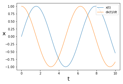
問題(単振動): ($k=1$はパラメータ)
$x''(t)+kx(t)=0$, 初期条件 $x(0)=0, x'(0)=1$

1階常微分方程式の問題では初期条件を数値で与えたが，2階以上の常微分方程式の解法では初期条件をリストで与えることに注意する。

コード

from sympy import *      # sympyライブラリから全ての機能をimoprt
import numpy as np      # numpyをnpという名前でimport 
from scipy.integrate import odeint 
import matplotlib.pyplot as plt
"""
2階微分方程式
例題 (単振動): d^2x/dt^2 = -kxを x(0)=0,x'(0)=1の初期条件の下で解く
"""
#シンボル定義
x=Symbol('x')                  # 文字'x'を変数xとして定義
t=Symbol('t')                  # 文字 't'を変数tとして定義
k=Symbol('k')                  # 文字 'k'を変数kとして定義。本問ではパラメータとして使う。
#

def func2(x, t, k):
    x1,x2=x
    dxdt=[x2,-k*x1]
    return dxdt

k = 1.0 # パラメータ設定
x0 = [0.0,1.0] # 初期条件: それぞれx(0), x'(0)を表す

t=np.linspace(0,10,101) # 積分の時間刻み設定: 0から10までを101等分する
sol2=odeint(func2, x0, t, args=(k,)) # 数値的に微分方程式を解き， x(t)とx'(t)をsol2のリストの[:,0]および[:,1]成分へ格納する。


#可視化

plt.plot(t, sol2[:,0], linewidth=1,label='x(t)') #  x(t) を図示
plt.plot(t, sol2[:,1], linewidth=1,label='dx(t)/dt') # dx/dt を図示
plt.xlabel('t', fontsize=18)
plt.ylabel('x', fontsize=18,rotation='horizontal')
plt.legend(loc='upper right')
plt.show()

結果