自動運転に必要な画像処理技術シリーズの3回目。今回は道路標識の認識です。今回も参照先は以下になります。
今回は上記で提供されるコードそのままではなく、Watson Studio独自の機能である、Neural Network Modelerを使用してみます。前半ではモデルを構築し、後半ではモデルを使って標識認識のアプリを作成します。
道路標識の認識
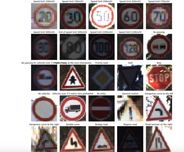
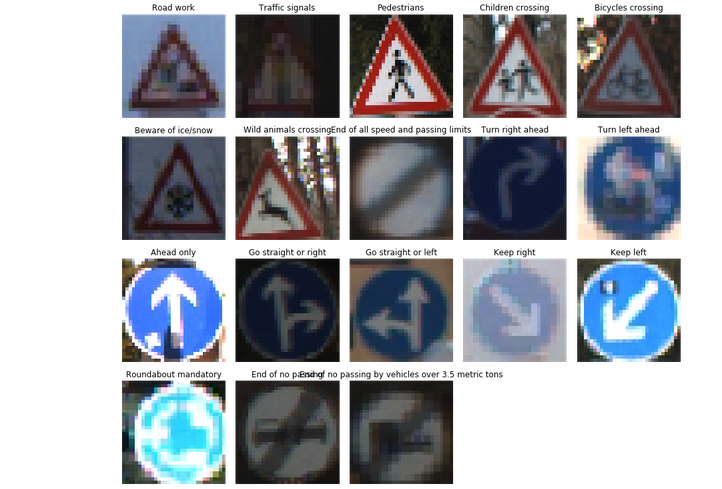
今回はこちらで公開されている、German Traffic Sign Dataset を使用します。以下のような道路標識の画像とそのクラス(43分類)のデータが提供されています。Neural Network Modeler作成したネットワークをこれらのデータで学習し、分類ができることをテストします。
手順
データの取得
データを取得し保管するためにIBM Cloud Object Storage(ICOS) にバケットを作成します。バケットの作成は以下等を参照してください。
Watson Studioでプロジェクトを作成して、以下リンク先から Notebook を作成します。
https://github.com/schiyoda/Self-Driving-Car/blob/master/3.1.Prepare-Data.ipynb
NotebookでICOSのcredentialとバケット名を指定した上で、全て実行すると、データをpickleに変換した上で、ICOSに保管されます。
Neural Networkの構築
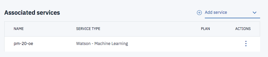
Watson Studioで適当なプロジェクトを作成します。プロジェクトのSettingsタブからWatson Machine Learningのサービスを紐付けておきます。
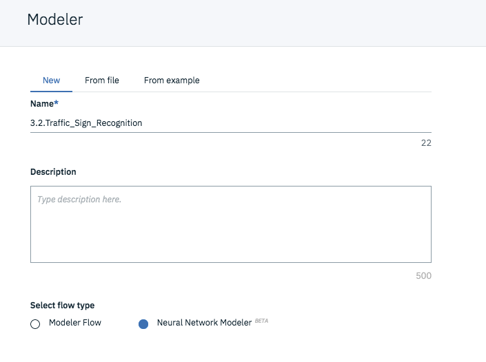
Assets タブに戻り、新規 Modeler Flow を作成します。
左側のパレットからNeural Networkの入力となる Image Data をドラッグ&ドロップします。
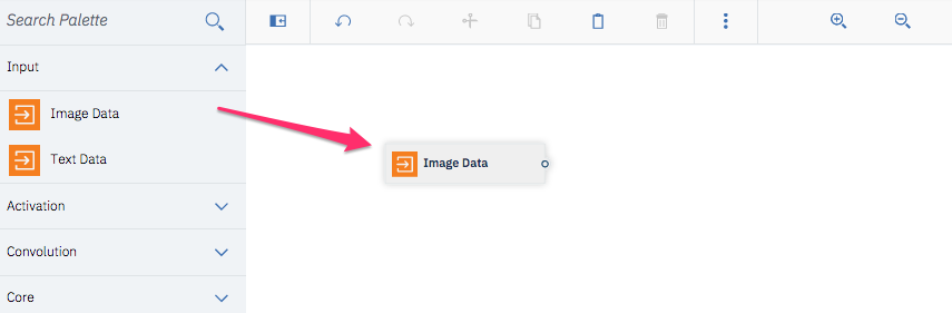
Image Data をダブルクリックすると右側にパネルが表示されるので以下のように設定します。
- Data Connections -> Connection to project COS(デフォルト)
- Backets -> 先の手順でpickleを保存したバケット
- Train data file -> training_data.pkl
- Image height, Image width -> 32, 32
- Classes -> 43
- Data format -> Python Pickle
- Epochs -> 50
Test data file, Validation data file を指定しないと、学習時にTrain dataを分割して Test, Validation に使用します。
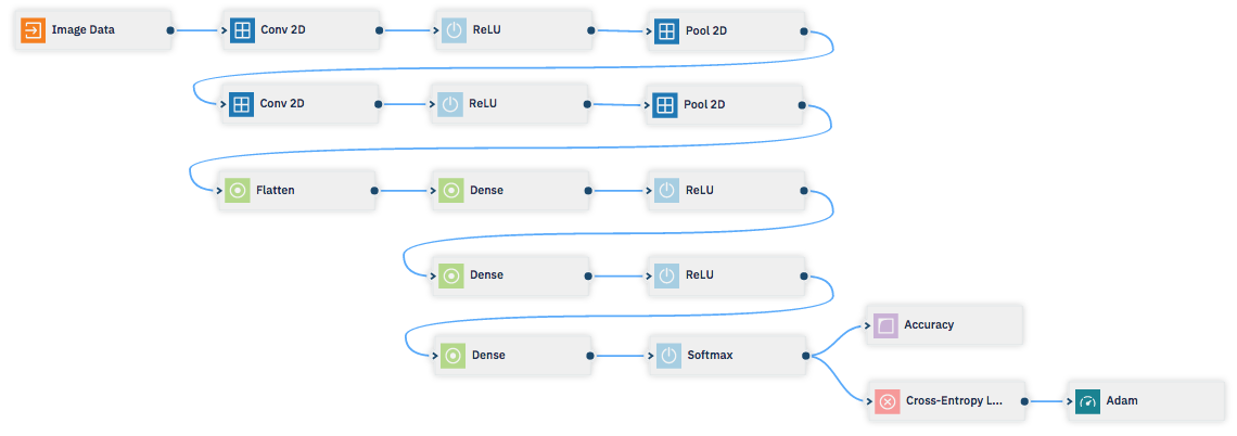
以降、以下のようにノードを配置してネットワークを構成します。
- Image Data(構成済み)
- Conv 2D
- Number of filters -> 6
- Kernel row, Kernel col -> 5, 5
- Weight LR multiplier,Weight decay multiplier -> 1, 1
- Bias LR multiplier, Bias decay multiplier -> 1, 1
- ReLU
- Pool 2D
- Kernel row, Kernel col -> 2, 2
- Stride row, Stride col -> 2, 2
- Conv 2D
- Number of filters -> 16
- Kernel row, Kernel col -> 5, 5
- Weight LR multiplier,Weight decay multiplier -> 1, 1
- Bias LR multiplier, Bias decay multiplier -> 1, 1
- ReLU
- Pool 2D
- Kernel row, Kernel col -> 2, 2
- Stride row, Stride col -> 2, 2
- Flatten
- Dense
- #nodes -> 120
- ReLU
- Dense
- #nodes -> 84
- ReLU
- Dense
- #nodes -> 43
- Softmax
- Accuracy, Cross-Entropy Loss (Softmaxから2箇所に繋ぐ)
- Adam
- Learning rate -> 0.01
完成したネットワークは以下のようになります。
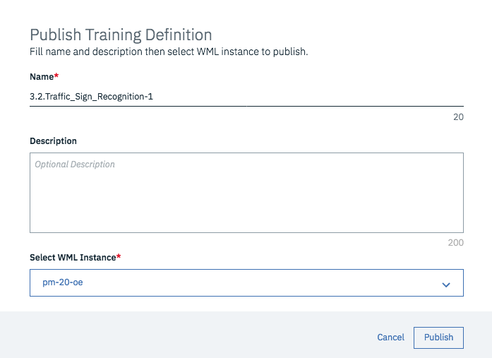
右上の をクリックし、training definition として publish します。
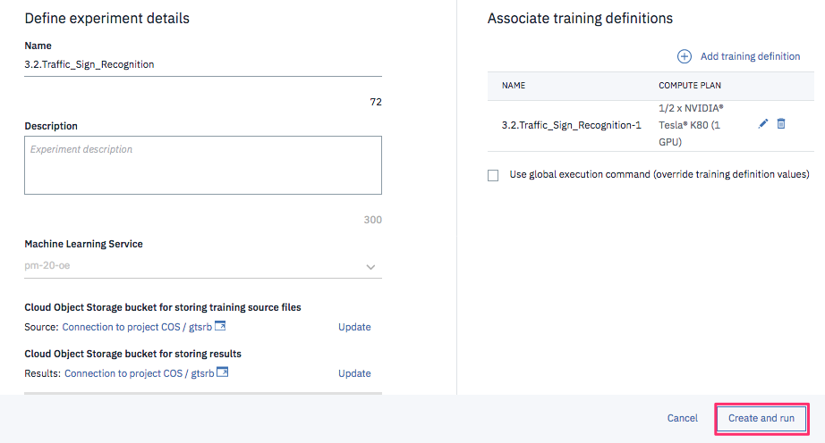
プロジェクトのページに戻り、新規 Experiment を作成します。
Cloud Object Storage bucket for storing training source files、Cloud Object Storage bucket for storing results には Existing connectionsから先の手順で作成した既存のバケットを選択します。
Add training definition では Existing training definition から先の手順で publish した training definition を選択します。
Compute plan は K80(1GPU)を選択します。
設定が完了したら以下の画面で Create and run をクリックし、学習を開始します。
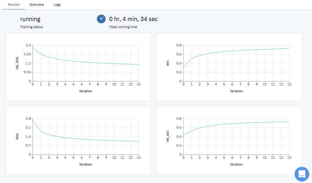
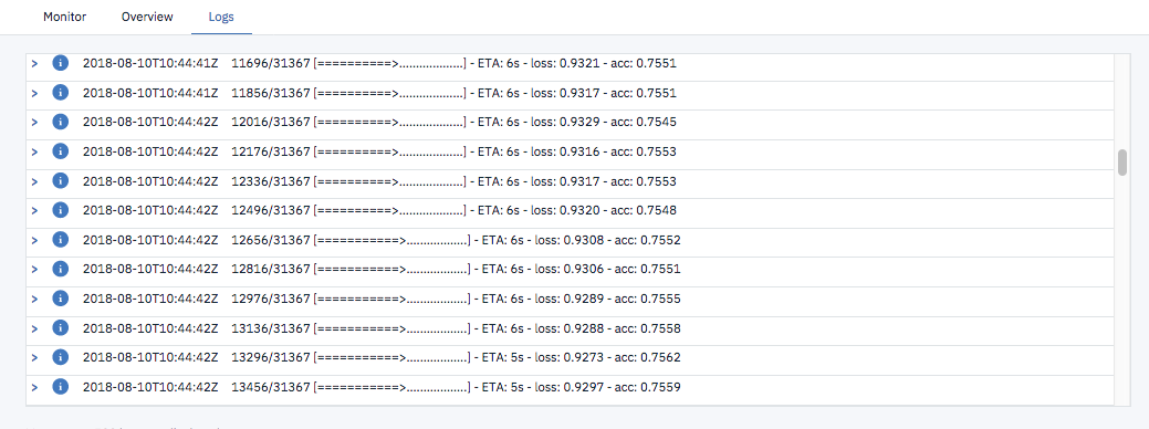
学習が開始すると、以下のよう学習曲線や実行のログや参照可能です。
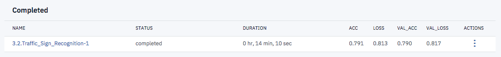
学習が完了するとステータスが Completed となります。今回の学習の結果、79%くらいのAccuracyのモデルが構築できたことが分かります。
次回は、このモデルを使って標識認識のアプリを作成してみます。