Pythonで「カイ２乗分布の定理」を確かめてみる

カイ（χ）２乗分布に関して以下の定理が成り立ちます。

\begin{align}
\\
&【定理】\\
\\
&分散\sigma^2の同じ正規分布に従うn個の確率変数X_1, X_2, ..., X_nを考える。\\
\\
&\bar{X} = \frac{X_1 + X_2 + ... + X_n}{n}\\
\\
&さらに以下の和を考えるとき、\\
\\
&\chi^2 = \Bigl( \frac{X_1-\bar{X}}{\sigma} \Bigr)^2 + \Bigl( \frac{X_2-\bar{X}}{\sigma}  \Bigr)^2 +...+ \Bigl( \frac{X_n-\bar{X}}{\sigma}  \Bigr)^2\\
\\
&この確率変数\chi^2は自由度n-1の \chi^2 分布に従う。\\
\\
&またs^2を不偏分散とした時、簡単な計算で以下の等式が成り立つことがわかります。\\
\\
&\chi^2 = \frac{n-1}{\sigma^2} s^2 \qquad (1)\\
&\qquad \qquad  \qquad \qquad  \qquad \qquad  \qquad \qquad \qquad  \qquad \qquad \qquad \qquad \qquad \qquad \qquad \qquad  \qquad  \\
\end{align}

定理を確認する

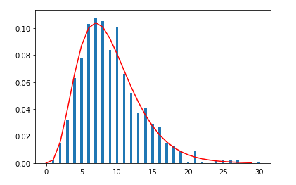
N(0,2)の正規分布に対してサイズ10の標本を取り出し不偏分散を計算する。それから(1)のカイ2乗を計算し棒グラフを描く。これが自由度9(=10-1)のカイ2乗分布で近似されていることをみる。

以下の簡単なPythonのプログラムを実行します。

import numpy as np
import matplotlib.pyplot as plt
from decimal import Decimal

# 1000個の標本に対して(1)を計算し棒グラフを描く
e={}
for i in range(1000):
    n = 10
    h = 2
    # 平均=loc=0.0, 標準偏差=scale=2, 個数=size=10
    a=np.random.normal(loc=0.0,scale=2, size=10)
    # 不偏分散の計算
    b = np.var(a, ddof=1)
    # χ２乗の計算
    c = ( (n-1)/(h*h) ) * b
    d = np.around(c, decimals=0)
    if d in e:
        e[d]=e[d]+1
    else:
        e[d]=1
es = sorted(e.items(), key=lambda x:x[0])
xs=[x for (x,y) in  es]
ys=[y/1000 for (x,y) in  es]
plt.bar(xs, ys, 0.35, linewidth=0)

# カイ２乗分布をプロットする
from scipy.stats import chi2
X = np.arange(0,30,1)
Y = chi2.pdf(X, df=9)
plt.plot(X,Y,color='r')

出力されたグラフを見ると、確かにカイ2乗分布で近似されているのがわかります。

今回は以上です。