Rで行う基本的な統計検定とその選択フローチャート2
このシリーズでは生物学で用いられている基本的な統計検定をRで行う際の手順と実際のコードを特集します。自身のデータセットの特徴と実験目的から適切な統計検定法を選択し、それをRで実行できるようになるための指針となれば幸いです。
第一回:平均値の差の検定(2群)
第二回:一元配置の分散分析
第三回:一元配置の多重比較
第四回:二元配置の分散分析とその後の多重比較
第五回:比率の差の検定
第六回:サンプルサイズの設計法
第七回:回帰分析
第三回 多重比較
3.1 適切な検定法の選択
フローチャート
3.2 パラメトリック多重比較
3.2.1 Bonferroni method
3.2.2 Holm method
3.2.3 Dunnet method(cont群と各処理群との比較)
3.2.4 Tukey-Kramer test(2群の比較を全通り行う)
3.2.5 Scheffe's multiple comparison method(全ての対比を行う)
3.3 ノンパラメトリック多重比較
3.3.1 Steel's method(Dunnet methodのノンパラ版)
3.3.2 Steel-Dwass test(Tukey-Kramer methodのノンパラ版)
3.1 適切な検定法の選択
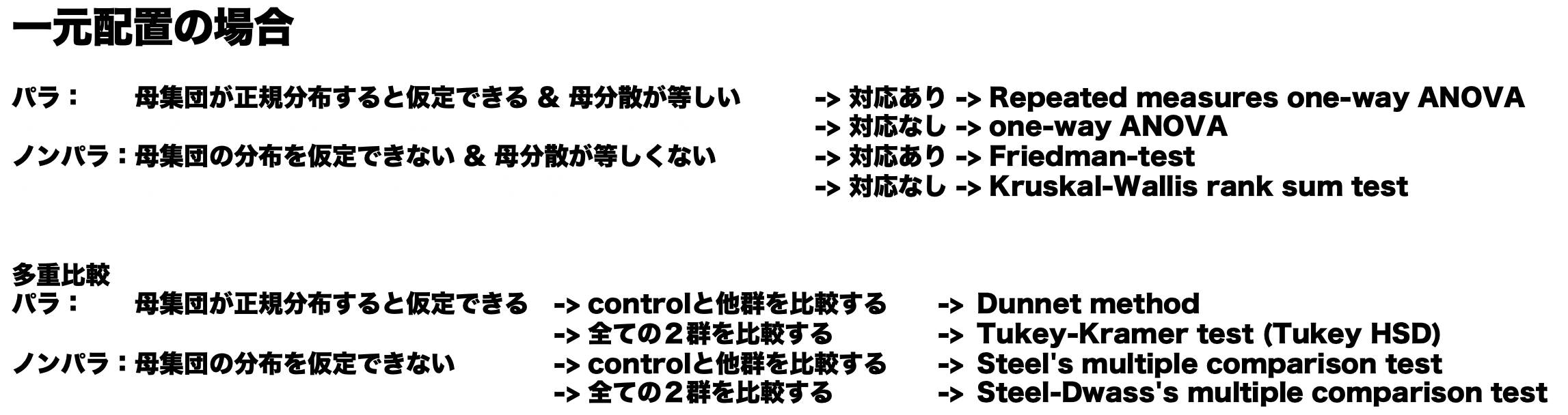
一元配置の実験デザインにおける平均値の差の多重比較の検定についてです。以下に検定法選択のためのフローチャートをのせておきます。選択の上で重要なのが、測定値について母集団が正規分布に従うと仮定できるか:正規性、を検証する必要があります。なおF統計量を用いる多重比較(Scheffe, Games/Howell, Fisher's PLSD)を使う場合は、事前にANOVAを行なって有意差があることを確認しておく必要があるが、F統計量を用いない多重比較法(Dunnet, Tukey-Kramer, Bonferroni)を使う場合は必ずしも事前のANOVAは必要でない。
検定法選択のためのフローチャート
3.2 パラメトリック多重比較
母集団が正規分布に従う&各群が等分散と仮定できる場合、パラメトリックな検定手法を使って、どの群に差があるか(多重比較)を検定することになります。この項では一般的な多重比較法を紹介する。
3.2.1 Bonferroni method
t 検定を使用してグループ平均の間でのペアごとの比較を行う。ただし、実験ごとのp値を総検定数で割った値を各検定のp値として設定することによって、全体のp値を調整する。Bonferroni補正を行うと有意水準が厳しくなりすぎると言われているため、群が増えると検出力が下がるので5群以上には適用すべきでない->改良したのがHolm法らしい
Rで実行してみよう。帰無仮説(H0)は各群の平均値はそれぞれの群間で等しいこと。
score = c(56, 48, 72, 60, 55, 60, 62, 76, 84, 78, 53, 62, 44, 90, 57, 77, 72, 83, 81, 91, 83)
class = factor(rep(c("A", "B", "C", "D"), c(5, 4, 6, 6)))
pairwise.t.test(score, class, paired=F, p.adjust.method="bonferroni")
結果
Pairwise comparisons using t tests with pooled SD

data:  score and class

  A    B    C
B 0.83 -    -
C 1.00 1.00 -
D 0.03 1.00 0.13

P value adjustment method: bonferroni
以上からA-Dについて帰無仮説は棄却され、A群とD群の間には平均値の差があると考えられる。
なおbonferroni methodはノンパラメトリックなデータにも適用可能で、その場合は
pairwise.wilcox.test(score, class, paired=F, p.adjust.method="bonferroni")
とする。これらは本質的にはt-testあるいはwilcoxon-testを繰り返して、bonferroniの方法でp値を補正するという考え方をするため、Rではt-testあるいはwilcoxon-testのオプションとしてp.adjust.method="bonferroni"を引数として指定している。
参照:https://data-science.gr.jp/implementation/ist_r_multiple_comparison_correction.html
3.2.2 Holm method
Bonferroni法を少し緩くした手法。参照↓
https://www.med.osaka-u.ac.jp/pub/kid/clinicaljournalclub1.html
score = c(56, 48, 72, 60, 55, 60, 62, 76, 84, 78, 53, 62, 44, 90, 57, 77, 72, 83, 81, 91, 83)
class = factor(rep(c("A", "B", "C", "D"), c(5, 4, 6, 6)))
pairwise.t.test(score, class, paired=FALSE, p.adjust.method="holm")
結果
Pairwise comparisons using t tests with pooled SD

data:  score and class

  A    B    C
B 0.55 -    -
C 0.81 0.81 -
D 0.03 0.55 0.11

P value adjustment method: holm
以上から帰無仮説は棄却され、bonferroni methodと同様、A群とD群の間には平均値の差があると考えられる。
なおholmの補正方法もノンパラメトリックなデータにも適用可能であり、
pairwise.wilcox.test(score, class, paired=FALSE, p.adjust.method="holm")
で実行することができる。
3.2.3 Dunnett method(cont群と各処理群との比較)
Dunnet methodは正規性の仮定が妥当である分布からサンプリングされた全ての処理群を対照群と同時に比較するための多重比較手順において広く使われている。
参照:https://ja.wikipedia.org/wiki/ダネットの検定
Rで実行してみる。帰無仮説(H0)はcont群と各処理群の各2群間の平均値に差がないことである。
なお群の名前のアルファベット順で最も若い群をcont群として認識するようなので、control群は"A"などとしておくのがよさそう。
install.packages("multcomp", repos="http://cran.ism.ac.jp/")
library(multcomp)
score = c(56, 48, 72, 60, 55, 60, 62, 76, 84, 78, 53, 62, 44, 90, 57, 77, 72, 83, 81, 91, 83)
class = factor(rep(c("A", "B", "C", "D"), c(5, 4, 6, 6)))
summary(glht(aov(score~class), linfct=mcp(class="Dunnett")))
結果
Simultaneous Tests for General Linear Hypotheses

Multiple Comparisons of Means: Dunnett Contrasts


Fit: aov(formula = score ~ class)

Linear Hypotheses:
           Estimate Std. Error t value Pr(>|t|)
B - A == 0   12.300      7.902   1.557   0.3055
C - A == 0    5.800      7.132   0.813   0.7544
D - A == 0   22.967      7.132   3.220   0.0133 *
---
Signif. codes:  0 ‘***’ 0.001 ‘**’ 0.01 ‘*’ 0.05 ‘.’ 0.1 ‘ ’ 1
(Adjusted p values reported -- single-step method)
以上からA-Dについて帰無仮説は棄却され、A群とD群の間には平均値の差があると考えられる。
3.2.4 Tukey-Kramer test(2群の比較を全通り行う)
各群の母集団が正規分布すると仮定されるときに、2群の比較を全通り行う検定法。しばしば分散分析と併用される。しかし実際にはF統計量を使用しないので、事前に分散分析を行う必要はない(分散分析で有意差が出ない場合でもTukey-Kramer testで有意差が出る場合がある)。
Rで実行してみよう。帰無仮説(H0)は各群の平均値はそれぞれの群間で等しいこと。
R
score = c(56, 48, 72, 60, 55, 60, 62, 76, 84, 78, 53, 62, 44, 90, 57, 77, 72, 83, 81, 91, 83)
class = factor(rep(c("A", "B", "C", "D"), c(5, 4, 6, 6)))
TukeyHSD(aov(score ~ class))
結果
Tukey multiple comparisons of means
    95% family-wise confidence level

Fit: aov(formula = score ~ class)

$class
        diff        lwr      upr     p adj
B-A 12.30000 -10.160603 34.76060 0.4278534
C-A  5.80000 -14.474534 26.07453 0.8474017
D-A 22.96667   2.692133 43.24120 0.0235201
C-B -6.50000 -28.112726 15.11273 0.8275432
D-B 10.66667 -10.946059 32.27939 0.5145020
D-C 17.16667  -2.164343 36.49768 0.0916375
以上よりA-Dについて帰無仮説は棄却され、A群とD群の間には平均値の差があると考えられる。
3.2.5 Scheffe's multiple comparison method
母集団は正規分布、各郡の母分散は等しい、各群のデータ数が異なる場合に適用できる。またF統計量を使うためANOVAで有意差が出ていないと有意差が出ない。また他の多重比較法では特定の2群間の比較を繰り返し行うが、本法では複数の群をまとめた群の比較など可能な全ての対比を行える(A vs B+C+DとかA+C vs B+Dとか)が、検出力は低くなる。二元配置のデータの因子ごとの多重比較にも適用が可能(多分)
Rで実行してみよう。帰無仮説(H0)は比較する群間の母平均は等しいこと。
score = c(56, 48, 72, 60, 55, 60, 62, 76, 84, 78, 53, 62, 44, 90, 57, 77, 72, 83, 81, 91, 83)
class = factor(rep(c("A", "B", "C", "D"), c(5, 4, 6, 6)))
library(agricolae)
dat=data.frame(score, class)
scheffe.test(aov(score ~ class, data=dat), "class", group=TRUE, console=TRUE)
結果
Study: aov(score ~ class, data = dat) ~ "class"

Scheffe Test for score

Mean Square Error  : 138.7431

class,  means

     score       std r Min Max
A 58.20000  8.843076 5  48  72
B 70.50000 11.474610 4  60  84
C 64.00000 17.005881 6  44  90
D 81.16667  6.400521 6  72  91

Alpha: 0.05 ; DF Error: 17
Critical Value of F: 3.196777

Groups according to probability of means differences and alpha level( 0.05 )

Means with the same letter are not significantly different.

     score groups
D 81.16667      a
B 70.50000     ab
C 64.00000     ab
A 58.20000      b
この結果が何を表すかはよくわからない笑(調査中)
参照:https://rdrr.io/cran/agricolae/man/scheffe.test.html
https://github.com/myaseen208/agricolae/blob/master/R/scheffe.test.R
3.3.2 ノンパラメトリック多重比較
母集団が正規分布に従わない、または各群が等分散でない場合、パラメトリックな検定手法を使って、どの群に差があるか(多重比較)を検定することになります。この項では一般的なノンパラ多重比較法を紹介する。
なおBOnferroni methodとHolm methodはノンパラデータにも適用できることは2.2.2.1と2.2.2.2で既に述べたので、それ以外の手法を紹介する。
3.3.1 Steel's method(Dunnet methodのノンパラ版)
Dunnet methodのノンパラ版、contと処理群の比較を繰り返す。
参照:http://aoki2.si.gunma-u.ac.jp/R/Steel.html
帰無仮説(H0)はcont群と各処理群の各2群間の値の分布に差がないことである。
が、しかし、Rで良さげなパッケージは見つからなかった。
青木先生の関数が存在するが、p値を自分で計算しないといけない。
参照:http://aoki2.si.gunma-u.ac.jp/R/Steel.html
また自作の関数でp値を出すようなものが見つかったが、入力するデータ型がいまいちわからなかったのと、うまく関数自体が動かなかった。
参照:https://www.trifields.jp/introducing-steel-in-r-1637
https://note.com/eiko_dokusho/n/nf3eb1600246d
ということでRでSteel's methodは現状では使え無さそう!EZRでは使えそうなので参照にしてください->https://best-biostatistics.com/ezr/multiple-test.html
3.2.2 Steel-Dwass test(Tukey-Kramer methodのノンパラ版)
正規分布を仮定しない各群間を順位を用いて多重比較で調べる方法である。
参照:http://aoki2.si.gunma-u.ac.jp/R/Steel.html
Rで実行してみる。帰無仮説(H0)はcont群と各処理群の各2群間の値の分布に差がないことである。
なお第一群で指定した群をcont群として各処理群と比較するようである。
install.packages("NSM3")    #ミ ラーサイトを選択するようにでるが、Japanでok
library("NSM3")

score <- c(6.9, 7.5, 8.5, 8.4, 8.1, 8.7, 8.9, 8.2, 7.8, 7.3, 6.8, 9.6, 9.4, 9.5, 8.5, 9.4, 9.9, 8.7, 8.1, 7.8, 8.8,  5.7, 6.4, 6.8, 7.8, 7.6, 7.0, 7.7, 7.5, 6.8, 5.9, 7.6, 8.7, 8.5, 8.5, 9.0, 9.2, 9.3, 8.0, 7.2, 7.9, 7.8)
group <- rep(1:4, c(11, 10, 10, 11))

pSDCFlig(score, group, method="Monte Carlo")  # モンテカルロ法で近似(?)
pSDCFlig(score, group, method="Asymptotic")  # 漸近法で近似
pSDCFlig(score, group, method="Exact")        # 正確、Rで動かないかも
結果(モンテカルロ法)
Ties are present, so p-values are based on conditional null distribution.
Group sizes: 11 10 10 11
Using the Monte Carlo (with 10000 Iterations) method:

For treatments 1 - 2, the Dwass, Steel, Critchlow-Fligner W Statistic is 3.7904.
The smallest experimentwise error rate leading to rejection is 0.027 .

For treatments 1 - 3, the Dwass, Steel, Critchlow-Fligner W Statistic is -3.5921.
The smallest experimentwise error rate leading to rejection is 0.0432 .

For treatments 1 - 4, the Dwass, Steel, Critchlow-Fligner W Statistic is 1.8139.
The smallest experimentwise error rate leading to rejection is 0.5842 .

For treatments 2 - 3, the Dwass, Steel, Critchlow-Fligner W Statistic is -5.2978.
The smallest experimentwise error rate leading to rejection is 0 .

For treatments 2 - 4, the Dwass, Steel, Critchlow-Fligner W Statistic is -2.8946.
The smallest experimentwise error rate leading to rejection is 0.1632 .

For treatments 3 - 4, the Dwass, Steel, Critchlow-Fligner W Statistic is 4.7863.
The smallest experimentwise error rate leading to rejection is 0.0014 .
結果(漸近法)
Ties are present, so p-values are based on conditional null distribution.
Group sizes: 11 10 10 11
Using the Asymptotic method:

For treatments 1 - 2, the Dwass, Steel, Critchlow-Fligner W Statistic is 3.7904.
The smallest experimentwise error rate leading to rejection is 0.037 .

For treatments 1 - 3, the Dwass, Steel, Critchlow-Fligner W Statistic is -3.5921.
The smallest experimentwise error rate leading to rejection is 0.054 .

For treatments 1 - 4, the Dwass, Steel, Critchlow-Fligner W Statistic is 1.8139.
The smallest experimentwise error rate leading to rejection is 0.5742 .

For treatments 2 - 3, the Dwass, Steel, Critchlow-Fligner W Statistic is -5.2978.
The smallest experimentwise error rate leading to rejection is 0.001 .

For treatments 2 - 4, the Dwass, Steel, Critchlow-Fligner W Statistic is -2.8946.
The smallest experimentwise error rate leading to rejection is 0.171 .

For treatments 3 - 4, the Dwass, Steel, Critchlow-Fligner W Statistic is 4.7863.
The smallest experimentwise error rate leading to rejection is 0.004 .
以上から
モンテカルロ法では、帰無仮説は1群-2群、1群-3群、2群-3群、2群-4群で棄却できず、これら対比群の値の分布に差があるとはいえない。
漸近法では帰無仮説は1群-2群、2群-3群、2群-4群で棄却できず、これら対比群の値の分布に差があるとはいえない。
モンテカルロ法と漸近法では1群-3群について帰無仮説の採択に差がでた。これは近似法の違いによる結果であろう。
なお正確法のコードを動かしてみたが、うまく処理されなかった。
青木先生のHPは漸近法で近似した手法が記載されている、参照:HP(http://aoki2.si.gunma-u.ac.jp/R/Steel-Dwass.html)
その他参照:https://biolab.sakura.ne.jp/steel-dwass.html
https://jojoshin.hatenablog.com/entry/2016/05/29/222528