Pythonで主成分分析して相関行列を可視化する

前提

・ある曲のサビ30秒間を抽出してメル周波数ケプストラム分析をする。
・２曲間のKLダイバージェンスを求める。
・↑視覚化する
・主成分分析したものを視覚化する
・相関行列になっていれば成功

データ

AKB48のフライングゲットとヘビーローテーションを比較する。

求めたKLダイバージェンスは16×16次元

[[  95.31099625   91.15557772   56.59372546  112.20285226   94.41219084
   211.66976101   92.55439072  121.40280516   99.87466514   76.50081387
   176.93201868   91.81223113   85.27707457  105.14295556  125.49246929
   130.92378707]
 [  61.39054933   94.3470823    62.02704779  107.94425798  128.17543843
   309.20131854   90.24173322  107.68055813  109.89023764   50.34427017
   223.12270163   86.42437451   56.75452679  147.27774644  140.3949859
   183.75894278]
 [ 105.66621666   82.44161726   55.37485991   95.92704467   71.93089191
   139.99784461  103.5305553   104.49783045  101.97799459   97.42010348
   125.64532251   93.76049908   96.99409273   81.04788291  101.66325191
   106.66200182]
 [  72.58173889   88.12377418   61.89530358   86.95335195  138.72571321
   312.35785101   90.41438615  113.71909706  118.77928154   65.50818774
   214.00175004  113.10626452   52.0092669   135.97299857  148.63792688
   193.27541302]
 [  81.63626278   89.21027233   65.00120995  130.11972589   98.52470863
   225.72264868   91.47807602  108.48086909   82.19549295   60.1953677
   178.25090454   74.23288462   86.75234338  119.57743314  121.44196645
   130.71085354]
 [ 112.80955973   84.20293672   66.13356741  126.27130948   60.46044078
   108.98487829   94.30643082  114.27767382   85.12283233  100.1694529
   123.12525354   77.02509766  127.07893463   77.72584545   90.34136209
    77.31272758]
 [  98.67181854   79.9882436    60.27699343   95.48883179   57.14726547
   106.75881027   84.51898243  105.15391427   96.42217442  103.36893403
   115.31304902   81.72145888  113.92827284   70.10342339   79.76864038
    85.59532391]
 [ 124.00540056  102.49330066   69.46940492  117.7972943    65.92281076
   122.42686859  109.21028055  139.69386525  120.41384311  124.96030812
   147.40336555   98.98037785  136.61224331   82.25578681  101.68799841
   101.60176282]
 [ 141.02536187   88.11442192   69.53316552  123.67378376   67.97351381
   111.42573997  108.78252174  128.35881238  103.34373259  117.07395769
   122.29312541  102.2082161   129.57301791   78.33587137  110.68395808
    89.29850647]
 [ 105.83495569   71.55826188   60.84049422   93.8003492    77.06177205
   150.83061505   86.87908254  114.92215578  100.28873519   90.46477627
   134.67789323   96.1906124    94.92596407   79.28705749  103.96680059
   107.35708818]
 [ 166.21174246  116.41752126   94.20800055  148.72009053   61.35802568
    82.62043669  132.79504129  158.40382344  130.28234204  168.90800616
   131.6410988   114.45081907  191.85294161   84.81226445  106.30195098
    89.39215458]
 [  65.41033607   67.36512259   45.30766447   70.95585215   66.52775288
   140.37168343   69.72982884   81.57225523   87.82282686   67.15724897
   121.30574971   69.68125315   67.9074851    76.44269754   77.95359039
    98.47073341]
 [  93.18094019   77.11815575   56.16982799   74.68534181   85.72265797
   159.071974     86.2112096   110.31931314  105.62643628   95.54275032
   131.41625514  110.34370673   79.29159169   78.66368263  104.24385502
   122.82713447]
 [ 151.91835442   95.8700754    78.95950183  106.69723914   66.8965109
    83.65254447  116.18496042  145.24555922  122.32195846  154.69915632
   107.94328396  128.95019683  145.70673878   67.11698712  105.83368936
    95.34869169]
 [  77.74571566   68.14642544   49.52404341   90.78773066   80.01443641
   181.90010793   78.31102815   87.9577934    82.56031457   62.65435512
   139.59025763   74.27213077   71.97330552   91.39001379   99.40086861
   112.40496471]
 [  80.29039282   80.71088572   58.43570222  109.4784385    67.87835361
   153.32727136   84.13107423   99.60128605   93.34917358   74.31430677
   147.10640919   65.51538298   99.68106666   93.5848086    87.98955945
    99.60590161]]

視覚化

ヒートマップで描画する。
グラフをきれいに表示できるseabornというライブラリを使う。

※タイトルが文字化けしたので日本語化する必要がある
site-packages/seaborn/rcmod.pyを編集

def set(context="notebook", style="darkgrid", palette="deep", font="Hiragino Kaku Gothic Pro", font_scale=1, color_codes=False, rc=None):

fontの部分を日本語フォントに変えればよい。

KLダイバージェンスをそのまま可視化する

# 16×16次元のデータ
KLD = [  95.31099625   91.15557772   56.59372546  112.20285226   94.41219084
   211.66976101   92.55439072  121.40280516   99.87466514   76.50081387
   176.93201868   91.81223113   85.27707457  105.14295556  125.49246929
   130.92378707]
 [  61.39054933   94.3470823  ...


import seaborn as sns
import matplotlib.pyplot as plt

# X軸Y軸に表示する文字列
feature_names = ['%d' % i for i in range(KLD.shape[1])]

# 可視化
sns.heatmap(KLD, annot=False, xticklabels=feature_names, yticklabels=feature_names)

plt.show()

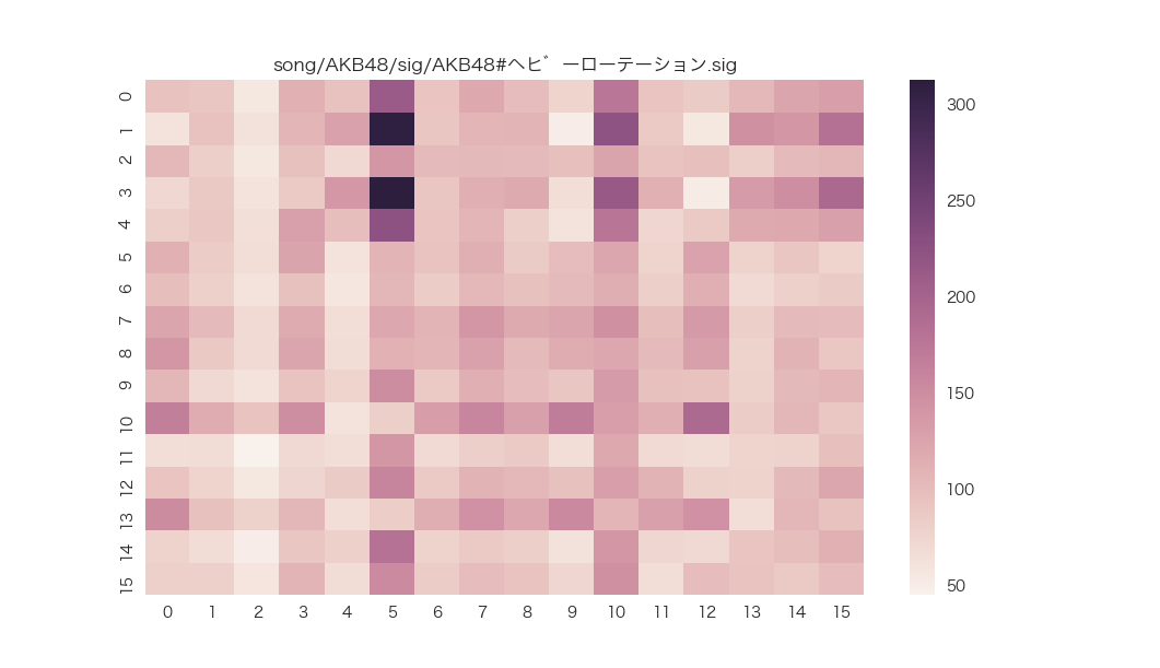
主成分分析していないので法則性がない。

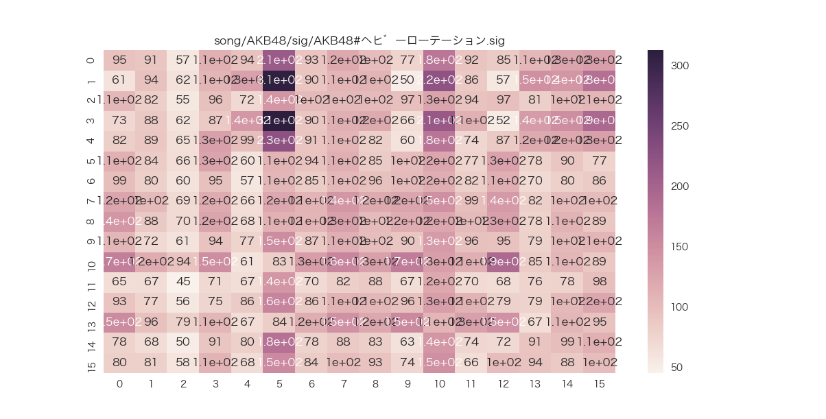
各次元での値も出力してみる。

# annotをTrueにすればOK
sns.heatmap(KLD, annot=True, xticklabels=feature_names, yticklabels=feature_names)

主成分分析して相関行列を可視化する

PCAという手法を使う

from sklearn.decomposition import PCA
import numpy as np

# n_componentsを指定しないとデータの次元数のまま分析される
pca = PCA()
pca.fit(KLD)
features = pca.fit_transform(KLD)
matrix = np.corrcoef(features.transpose())

sns.heatmap(matrix, annot=True, xticklabels=feature_names, yticklabels=feature_names)

plt.show()

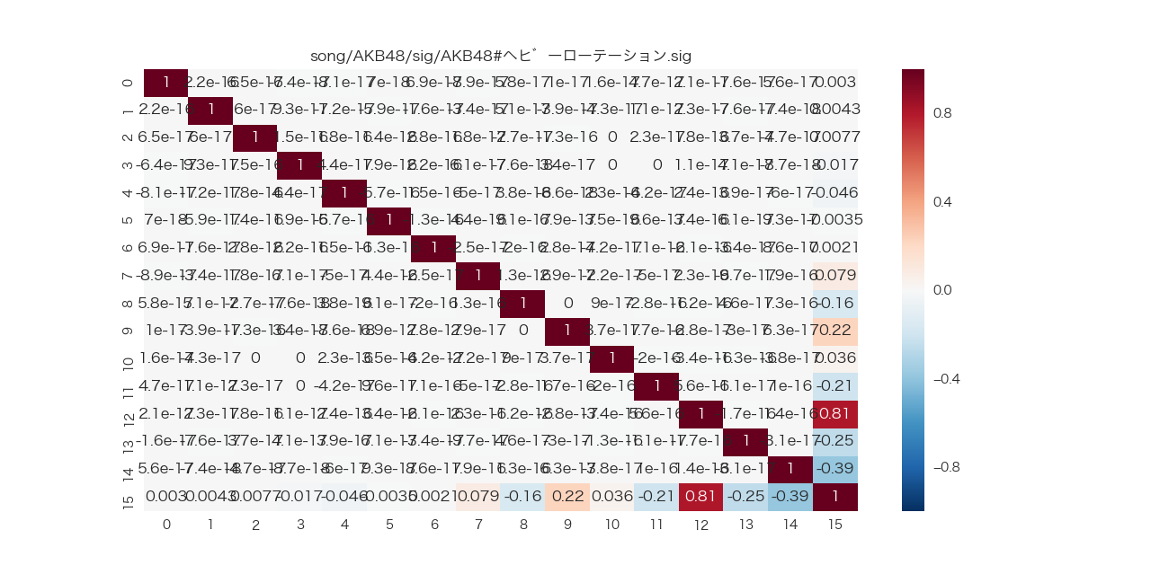
対角成分がちゃんと全部1になった！
相関行列の特徴を満たしている。

次元圧縮して主成分分析して可視化する

上記はそのまま16×16次元で主成分分析を行ったが
16×16だとさすがに多いので5×5に次元を落とす。

#n_componetsが次元数となる
pca = PCA(n_components=5)

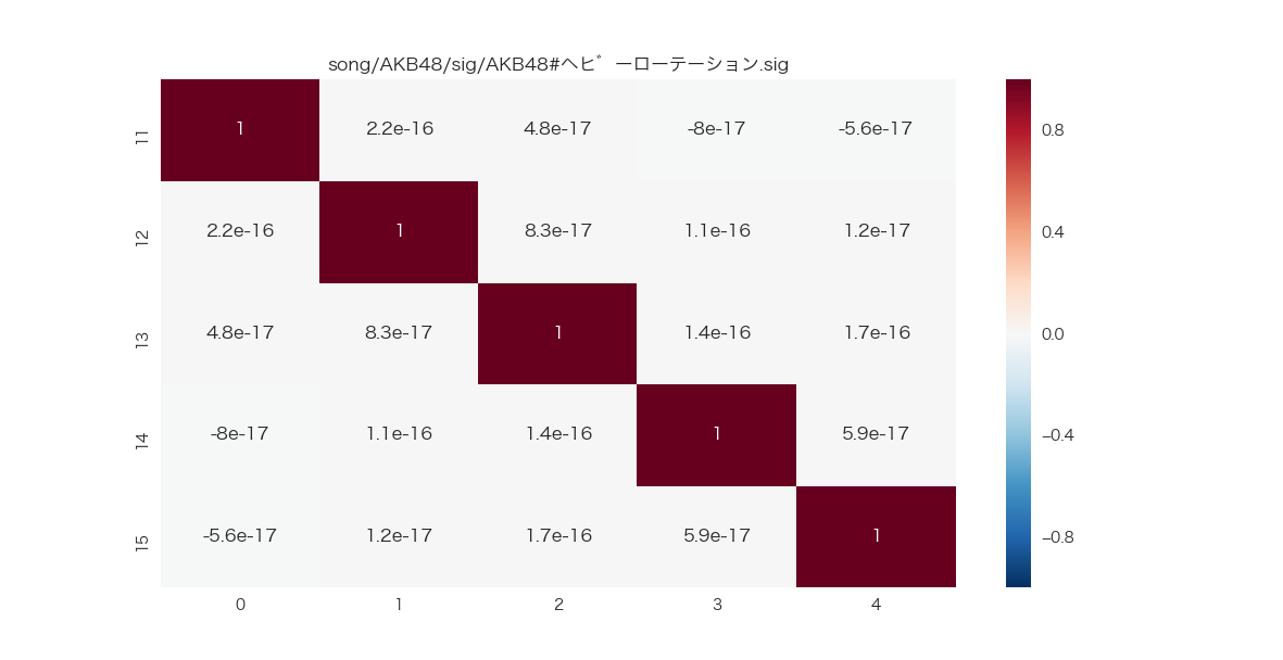
見やすい。