FinCEN文章を解析する_02（年別の時間変化）

FinCEN文章を解析する_02（各国の時間変化）

第一回：https://qiita.com/s_zh/items/b7c7eb7bc2af98b850d7

内容について

前回の記事で全期間中の各金融機関のなどの状況を解析したり、国別でデータを見ましたが、今回は年単位で各国の状況を見てみます。目標は各国の送金関係の時間変化を可視化することです。今回はその前処理として、まず各国の送金の時間変化についておおよその状況を掴みます。

ソースコードはこちらになります。

Colabに上げてNeo4j Sandboxと組み合わせればブラウザだけで解析することもできるはずです（ライブラリを適宜インストールする必要がありますが、必要な方はこちらの記事をご参照くださいhttps://qiita.com/s_zh/items/3b183e258bcd6506e8cb）

ライブラリ読み込み、データベースアクセスの準備

お約束の構文です。

import plotly.express as px
import numpy as np

from neo4j import GraphDatabase
from tqdm.notebook import tqdm
import json

import pandas as pd

auth_path = './data/neo4j_graph/auth.json'
with open(auth_path, 'r') as f:
    auth = json.load(f)

# ローカルの場合は通常 uri: bolt(or neo4j)://localhost:7687, user: neo4j, pd: 設定したもの
# サンドボックスの場合は作成画面から接続情報が見られます
uri = 'neo4j://localhost:7687'
driver = GraphDatabase.driver(uri=uri, auth=(auth['user'], auth['pd']))

# Sandboxの場合はこんな感じ
# uri = 'bolt://54.175.38.249:35275'
# driver = GraphDatabase.driver(uri=uri, auth=('neo4j', 'spray-missile-sizing'))

年別の傾向

年別のレコードを取得して集計します。送金額をamount、送金回数をcountとします。

with driver.session() as session:
    res = session.run('''
    MATCH (n:Filing)
    RETURN n.begin.year as year, sum(n.amount) as amount, count(n) as count
    ORDER BY year
    ''')

res_df = pd.DataFrame([r.data() for r in res])

res_df.shape

(18, 3)

送金量について見てみます。

px.bar(res_df, x='year', y='amount')

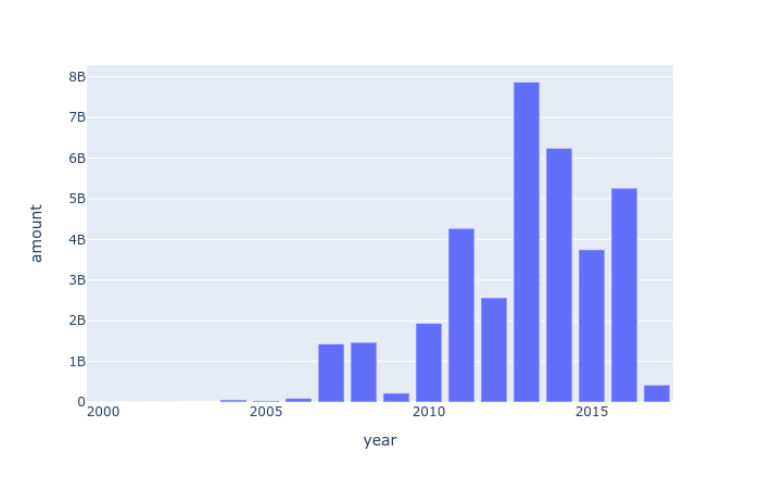
金融危機と同じ時期に急増しているのは興味深いですね。２００９年の急減はヨーロッパ通貨危機とかぶるのも何か関係があるのでしょうか。２０１３年にピークをつけているようです。

では送金回数を見てみましょう。

px.bar(res_df, x='year', y='count')

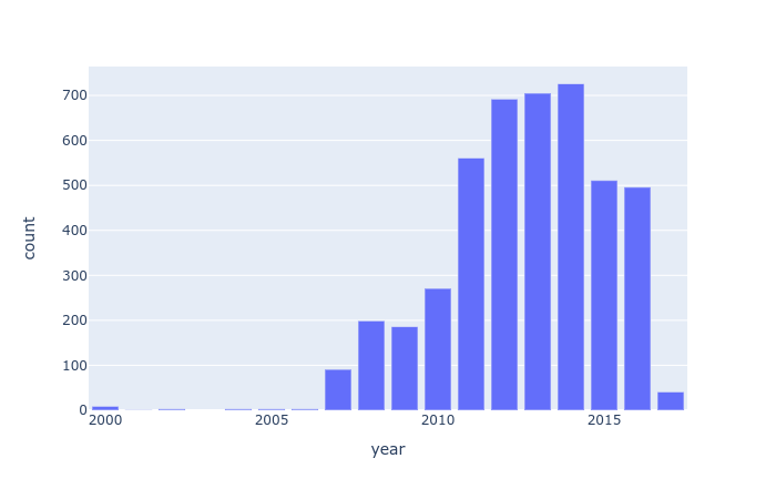
基本的に２０１４年までは増加傾向のようです。２００９年の金額の急落はお金がないから減ったのかな、２０１６年は件数が減っているのに金額が増えたのも実は潤っているからか、と邪推したくなりますね。

amount by country

国別に見てみましょう。国別の金額と回数の集計をします。

with driver.session() as session:
    res = session.run('''
    MATCH (n:Filing)-[:BENEFITS]-(:Entity)--(c:Country)
    RETURN c.name as country, n.begin.year as year, sum(n.amount) as amount, count(n) as count
    ORDER BY year
    ''')

日付のないデータを落とします。

res_df = pd.DataFrame([r.data() for r in res])
res_df.shape

(465, 4)

res_df = res_df.dropna()
res_df.shape

(460, 4)

国別、年別に集計します。

まずは金額から

res_df_country = res_df.groupby(['country']).sum()

res_df_country_order_by_amount = res_df_country.sort_values('amount', ascending=False)
res_df_country_order_by_amount

	year	amount	count
country
Russia	24138.0	7.279861e+09	486
Latvia	22132.0	3.947781e+09	498
Switzerland	24136.0	3.744860e+09	445
Singapore	22132.0	2.947456e+09	238
Hong Kong	20123.0	2.655467e+09	263
...	...	...	...
Jamaica	4020.0	1.942582e+04	2
Greece	2009.0	5.738450e+03	1
Jersey	2011.0	3.224220e+03	1
Colombia	2015.0	2.250000e+03	1
Romania	2014.0	9.000000e+02	1

107 rows × 3 columns

送金回数も同様です。

res_df_country_order_by_count = res_df_country.sort_values('count', ascending=False)
res_df_country_order_by_count

	year	amount	count
country
Latvia	22132.0	3.947781e+09	498
Russia	24138.0	7.279861e+09	486
Switzerland	24136.0	3.744860e+09	445
United States	28143.0	1.824221e+09	267
Hong Kong	20123.0	2.655467e+09	263
...	...	...	...
Puerto Rico	2015.0	1.670000e+05	1
Sri Lanka	2008.0	2.300000e+05	1
Qatar	2014.0	6.965325e+05	1
Romania	2014.0	9.000000e+02	1
Jersey	2011.0	3.224220e+03	1

107 rows × 3 columns

上位国の推移を見てみます。

country_list_amount = res_df_country_order_by_amount.index[:7]
country_list_count = res_df_country_order_by_count.index[:7]

金額の推移です。

res_df_filtered_by_country = res_df[res_df.country.isin(country_list_amount)]

px.line(res_df_filtered_by_country, x='year', y='amount', color='country')

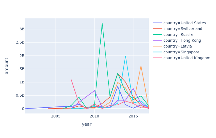
時間と共に大きく変化しています。ロシアへの送金は２０１１年に集中していて、その後は減少傾向です。一方でシンガポール、スウェーデン、ラトビアは近年増えています。

送金回数の推移です。

res_df_filtered_by_country = res_df[res_df.country.isin(country_list_count)]
px.line(res_df_filtered_by_country, x='year', y='count', color='country')

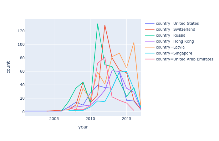
ラトビアは概ねトレンドを描いて上昇傾向であるように見えます。金額では目立たないUAEが浮上してきました。

これを時々見かける時間変化の動画にすると次のような感じになります。

Bar Chart Race

時間変化の動画を作るためのソースコードが下記です

information_format = {}
for rec in res_df.to_dict(orient='records'):
    country = rec['country']
    year = rec['year']
    amount = rec['amount']
    if not year:
        continue
    if country in information_format:
        information_format[country][year] = amount
    else:
        information_format[country] = {year: amount}

country_year_amount_df = pd.DataFrame(information_format)

country_year_amount_df = country_year_amount_df.sort_index().T

country_year_amount_df

	2000.0	2001.0	2002.0	2004.0	2005.0	2006.0	2007.0	2008.0	2009.0	2010.0	2011.0	2012.0	2013.0	2014.0	2015.0	2016.0	2017.0
Peru	5700446.06	NaN	NaN	NaN	NaN	NaN	1961821.00	NaN	NaN	NaN	NaN	NaN	1.801819e+05	2.904759e+05	3.625025e+06	3.044300e+07	NaN
United States	NaN	7769.89	NaN	54297237.53	NaN	83950000.0	79593802.00	1.680078e+08	4799923.17	81111267.42	7.504763e+07	2.865208e+07	8.391423e+08	1.491771e+08	1.721105e+07	1.478597e+08	95363351.00
Belarus	NaN	NaN	9402.0	NaN	NaN	NaN	NaN	NaN	NaN	NaN	NaN	NaN	NaN	NaN	3.958548e+07	NaN	NaN
Spain	NaN	NaN	NaN	20000.00	NaN	NaN	NaN	NaN	NaN	NaN	NaN	NaN	2.243146e+06	7.968587e+06	1.944970e+03	1.500000e+04	NaN
Switzerland	NaN	NaN	NaN	195000.00	NaN	NaN	18788349.56	1.042613e+08	44588788.40	38177154.77	1.990626e+08	4.396638e+08	1.328279e+09	1.004730e+09	4.415746e+08	1.183473e+08	7191512.77
...	...	...	...	...	...	...	...	...	...	...	...	...	...	...	...	...	...
Maldives	NaN	NaN	NaN	NaN	NaN	NaN	NaN	NaN	NaN	NaN	NaN	NaN	NaN	NaN	5.013589e+05	NaN	NaN
Puerto Rico	NaN	NaN	NaN	NaN	NaN	NaN	NaN	NaN	NaN	NaN	NaN	NaN	NaN	NaN	1.670000e+05	NaN	NaN
Saudi Arabia	NaN	NaN	NaN	NaN	NaN	NaN	NaN	NaN	NaN	NaN	NaN	NaN	NaN	NaN	4.793496e+07	1.528821e+07	NaN
Lao People's Democratic Republic	NaN	NaN	NaN	NaN	NaN	NaN	NaN	NaN	NaN	NaN	NaN	NaN	NaN	NaN	NaN	1.388230e+06	NaN
Uzbekistan	NaN	NaN	NaN	NaN	NaN	NaN	NaN	NaN	NaN	NaN	NaN	NaN	NaN	NaN	NaN	3.693000e+06	NaN

107 rows × 17 columns

country_year_amount_df.to_csv('./data/fincen/country_year_amount.csv')

このままだと国旗が表示されません。国旗を表示させるためには各国の国旗のURLを与える必要があります。

flags

country_flags = pd.read_csv('./data/country_flags.csv', header=None)
country_flags.columns = ['country', 'cotinent', 'flag']

country_flags = country_flags.set_index('country')

country_flags

	cotinent	flag
country
Angola	Africa	https://www.countryflags.io/ao/flat/64.png
Burundi	Africa	https://www.countryflags.io/bi/flat/64.png
Benin	Africa	https://www.countryflags.io/bj/flat/64.png
Burkina Faso	Africa	https://www.countryflags.io/bf/flat/64.png
Botswana	Africa	https://www.countryflags.io/bw/flat/64.png
...	...	...
Solomon Islands	Oceania	https://www.countryflags.io/sb/flat/64.png
Tonga	Oceania	https://www.countryflags.io/to/flat/64.png
Tuvalu	Oceania	https://www.countryflags.io/tv/flat/64.png
Vanuatu	Oceania	https://www.countryflags.io/vu/flat/64.png
Samoa	Oceania	https://www.countryflags.io/ws/flat/64.png

215 rows × 2 columns

country_year_amount_df.shape

(107, 17)

country_year_amount_df.join(country_flags)

	2000.0	2001.0	2002.0	2004.0	2005.0	2006.0	2007.0	2008.0	2009.0	2010.0	2011.0	2012.0	2013.0	2014.0	2015.0	2016.0	2017.0	cotinent	flag
Peru	5700446.06	NaN	NaN	NaN	NaN	NaN	1961821.00	NaN	NaN	NaN	NaN	NaN	1.801819e+05	2.904759e+05	3.625025e+06	3.044300e+07	NaN	Americas	https://www.countryflags.io/pe/flat/64.png
United States	NaN	7769.89	NaN	54297237.53	NaN	83950000.0	79593802.00	1.680078e+08	4799923.17	81111267.42	7.504763e+07	2.865208e+07	8.391423e+08	1.491771e+08	1.721105e+07	1.478597e+08	95363351.00	NaN	NaN
Belarus	NaN	NaN	9402.0	NaN	NaN	NaN	NaN	NaN	NaN	NaN	NaN	NaN	NaN	NaN	3.958548e+07	NaN	NaN	Europe	https://www.countryflags.io/by/flat/64.png
Spain	NaN	NaN	NaN	20000.00	NaN	NaN	NaN	NaN	NaN	NaN	NaN	NaN	2.243146e+06	7.968587e+06	1.944970e+03	1.500000e+04	NaN	Europe	https://www.countryflags.io/es/flat/64.png
Switzerland	NaN	NaN	NaN	195000.00	NaN	NaN	18788349.56	1.042613e+08	44588788.40	38177154.77	1.990626e+08	4.396638e+08	1.328279e+09	1.004730e+09	4.415746e+08	1.183473e+08	7191512.77	Europe	https://www.countryflags.io/ch/flat/64.png
...	...	...	...	...	...	...	...	...	...	...	...	...	...	...	...	...	...	...	...
Maldives	NaN	NaN	NaN	NaN	NaN	NaN	NaN	NaN	NaN	NaN	NaN	NaN	NaN	NaN	5.013589e+05	NaN	NaN	Asia	https://www.countryflags.io/mv/flat/64.png
Puerto Rico	NaN	NaN	NaN	NaN	NaN	NaN	NaN	NaN	NaN	NaN	NaN	NaN	NaN	NaN	1.670000e+05	NaN	NaN	Americas	https://www.countryflags.io/pr/flat/64.png
Saudi Arabia	NaN	NaN	NaN	NaN	NaN	NaN	NaN	NaN	NaN	NaN	NaN	NaN	NaN	NaN	4.793496e+07	1.528821e+07	NaN	Asia	https://www.countryflags.io/sa/flat/64.png
Lao People's Democratic Republic	NaN	NaN	NaN	NaN	NaN	NaN	NaN	NaN	NaN	NaN	NaN	NaN	NaN	NaN	NaN	1.388230e+06	NaN	NaN	NaN
Uzbekistan	NaN	NaN	NaN	NaN	NaN	NaN	NaN	NaN	NaN	NaN	NaN	NaN	NaN	NaN	NaN	3.693000e+06	NaN	Asia	https://www.countryflags.io/uz/flat/64.png

107 rows × 19 columns

country_year_amount_df.join(country_flags).to_csv('./data/fincen/country_year_amount_flag.csv')