この記事では、SIGNATE StudentCup2022Summerのデータサイエンティストの職種判別チャレンジの予測部門のデータについて探索的データ分析(Explanatory Data Analysis, EDA)を行います。
大まかに以下のことを行います。
- jobflagの内訳(Train)
- Train/Testの重複データ確認
- Train/Testデータの文字数比較
- Trainデータの職種別文字数比較
- 単語出現頻度分析
- 単語の出現に基づく職種の予測(ルールベース)
※2022/8/5修正
単語数比較と記載していたものが実際には文字数比較になっていたので、タイトルの修正を行いました。
import/初期設定
import numpy as np
import pandas as pd

import seaborn as sns
import matplotlib.pyplot as plt

import warnings
warnings.filterwarnings("ignore")

%matplotlib inline
sns.set_style("whitegrid")
plt.style.use("fivethirtyeight")
Train/Testデータの読み込み
DATA_DIR = "/content/drive/MyDrive/SIGNATE/studentcup2022summer/dataset/"
re_labels = {1: "DS", 2: "ML", 3:"SE", 4:"Cons"}
train = pd.read_csv(DATA_DIR + "train.csv")
train["jobflag"] = train["jobflag"].map(re_labels)
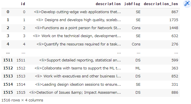
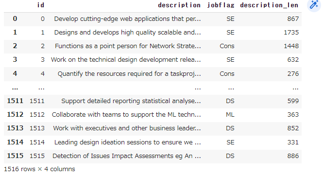
train['description_len'] = train["description"].apply(len) # descriptionの単語数
train#.head()
test = pd.read_csv(DATA_DIR + "test.csv")
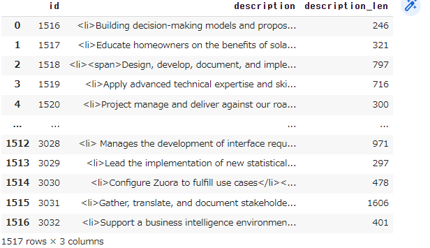
test['description_len'] = test["description"].apply(len)
test#.head()
jobflagの内訳(Train)
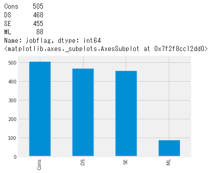
Trainデータ内のjobflagの頻度。Cons>DS>SE>MLの順に多い。
print(train["jobflag"].value_counts())
train["jobflag"].value_counts().plot(kind='bar')
Train/Testの重複データ確認
Train/Testを結合し、重複のあるデータを抽出する。Testデータの場合は橙色で塗りつぶしている。
def highlight_duplicate(val):
    if val["jobflag"] is np.nan:
        return ['background-color: orange']*len(val)
    else:
        return ['background-color: white']*len(val)

concat_train_test = pd.concat([train, test]).reset_index(drop=True)
duplicates = concat_train_test[concat_train_test["description"].duplicated(keep=False)].sort_values(by=["description","id"])

# Train/Testの両方に含まれているデータについて、Testデータの件数をカウントする
dup_between_train_and_test = 0
for flag in duplicates['description'].unique():
  tmp = duplicates[duplicates['description'] == flag]['jobflag']
  if tmp.isna().sum() > 0 and tmp.notna().sum() > 0:
    dup_between_train_and_test += tmp.isna().sum()
print(f"Duplication between Train and Test: {dup_between_train_and_test}")

duplicates.head(10).style.apply(highlight_duplicate, axis=1)

# Duplication between Train and Test: 27
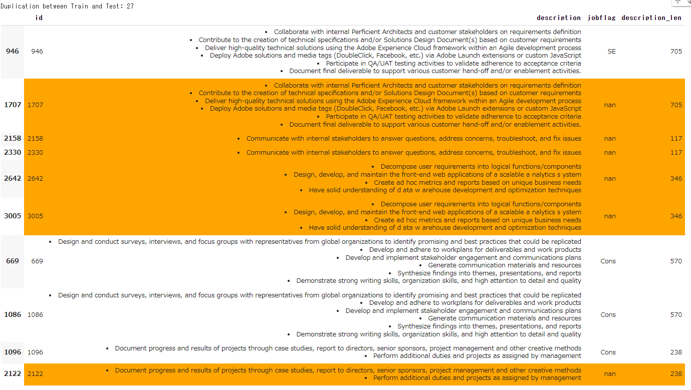
結果:
重複データとして抽出されたのは92件、そのうち、Train/Testの両方に含まれているTestデータの件数は27件あった。Trainデータをそのまま予測値とすることも出来るかもしれない。
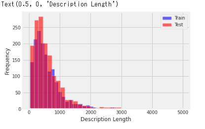
Train/Testデータの文字数比較
文字数の分布をヒストグラムにし、TrainとTestで重ねた図。概ね似た分布であることが分かる。
plt.figure(figsize=(6, 4))
train["description_len"].plot(bins=35, kind='hist', color='blue', label='Train', alpha=0.6)
test["description_len"].plot(bins=35, kind='hist', color='red', label='Test', alpha=0.6)
plt.legend()
plt.xlabel("Description Length")
Trainデータの職種別文字数比較
職種別の文字数を箱ひげ図によって示す。
sns.boxplot(x="description_len", y="jobflag", data=train,palette='rainbow')
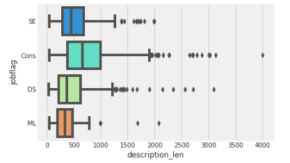
結果:
Consは他職種と比較するとやや文字数が多い求人が多くある。必要とされる能力の説明で長くなるのか、案件説明で長くなるのか。或いは、SE/ML/DSは必要とされる能力がピンポイントで言語化しやすいから短くなるのか、幾つか予測が立てられる。
単語出現頻度分析
nltkを用いて、名詞や固有名詞の単語の出現頻度を計算し、棒グラフやWordCloudで可視化した。最後に、各職種で特有に出現する単語の可視化も行っている。nltk参考
import nltk
from collections import Counter
from nltk.corpus import stopwords

nltk.download('all')
stopwords = list(stopwords.words('english'))

def repeated_word_count(text, target_pos=None):
    """text中の単語出現頻度を計算する"""
    morph = nltk.word_tokenize(text)
    poss = nltk.pos_tag(morph)
    words = []
    for pos in poss:
      if target_pos is None:
        words += [pos[0]]
        continue
      if pos[1] in target_pos and pos[0] not in stopwords:
        words += [pos[0]]

    word_counts = Counter(words)
    return words, word_counts
前処理として、Trainデータに対してhtmlタグ、.,/'’、&などの特殊文字の除去を行った。なお今回、大文字・小文字の単語を分かりやすくするためにこれらの統一は行わない。
import re
p = re.compile(r"<[^>]*?>|&|[.,/'’\"”]")
preprocess_train = train.copy()
preprocess_train['description'] = preprocess_train['description'].map(lambda x: p.sub("", x))
preprocess_train['description'] = preprocess_train['description'].map(lambda x: x.lstrip())
preprocess_test = test.copy()
preprocess_test['description'] = preprocess_test['description'].map(lambda x: p.sub("", x))
preprocess_test['description'] = preprocess_test['description'].map(lambda x: x.lstrip())
# preprocess_train
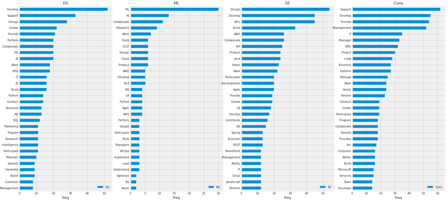
名詞の出現頻度の可視化
各職種ごとに単語の出現頻度を集計し、頻度が上位30個の単語を可視化した。
from wordcloud import WordCloud

def visualize_word_freq(text, target_pos, top_n=3):
  _, word_count = repeated_word_count(text, target_pos)
  pd.Series(word_count).sort_values(ascending=False)[:top_n][::-1].plot(kind='barh', label=str_flag)
  ax.legend()
  ax.set_title(str_flag)
  ax.set_xlabel("Freq")
  ax.tick_params()
  return fig, ax

def visualize_word_cloud(text, target_pos, top_n=30):
  words, _ = repeated_word_count(text, target_pos=target_pos)
  wordcloud = WordCloud(background_color="white")
  wordcloud.generate(" ".join(words))
  ax.set_title(str_flag)
  ax.tick_params(labelbottom=False,
              labelleft=False,
              labelright=False,
              labeltop=False)
  ax.imshow(wordcloud)
  return fig, ax
fig = plt.figure(figsize = (24, 12))
for i, str_flag in re_labels.items():
  ax = fig.add_subplot(1, 4, i)
  text = " ".join(preprocess_train[preprocess_train["jobflag"] == str_flag]["description"])
  _ = visualize_word_freq(text, target_pos=["NN", "NNS"], top_n=30) # NN:名詞, NNS:名詞複数形
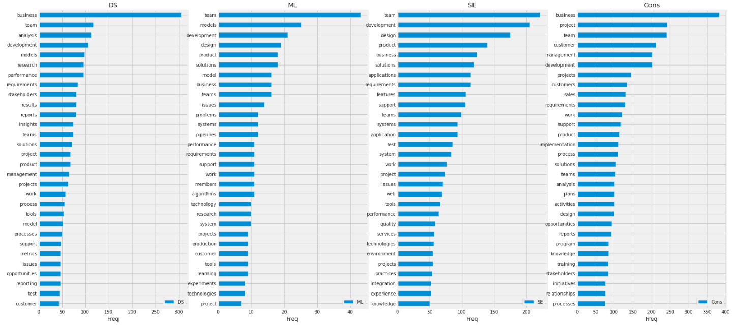
結果:
全職種で、team、business、developmentなど職種に寄らず比較的共通する単語が上位に入っていた。MLはmodelやalgorithms、SEではapplicationsなど技術的な内容を示唆する単語が見受けられた。Consでは、customersやmanagement、salesなど経営や管理などの視点に立った単語が観察され、先ほどML/SEで上げた単語は入っていなかった。DSでは、MLとConsを合わせたような単語が見受けられた。
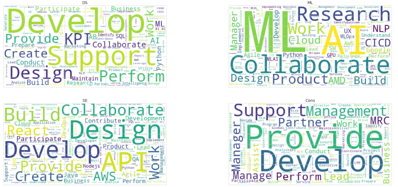
WordCloud図。どの職種でも、team, businessm, project等抽象的な単語が目に付く。
fig = plt.figure(figsize = (24, 12))
for i, str_flag in re_labels.items():
  ax = fig.add_subplot(2, 2, i)
  text = " ".join(preprocess_train[preprocess_train["jobflag"] == str_flag]["description"])
  _ = visualize_word_cloud(text, target_pos=["NN", "NNS"], top_n=30)

固有名詞の出現頻度の可視化
各職種ごとに固有名詞の出現頻度を集計し、頻度が上位30個の単語を可視化した。
fig = plt.figure(figsize = (24, 12))
for i, str_flag in re_labels.items():
  ax = fig.add_subplot(1, 4, i)
  text = " ".join(preprocess_train[preprocess_train["jobflag"] == str_flag]["description"])
  _ = visualize_word_freq(text, target_pos=["NNP", "NNPS"], top_n=30) # NN:固有名詞, NNS:固有名詞複数形
結果:
名詞の時に比べて全職種で差があった。MLではAIやML、NLPなど実際の業務に関わりそうな単語が見られた。SEではAPIやAWS、Java、Reactなどシステム開発よりの単語が見受けられた。DSでは、MLやAI等に加え、Consで一位になっているSupportの単語が上位に入っていた。(Supportが固有名詞は微妙。大文字小文字統一をしていなかったため、文の先頭に来る単語が固有名詞として数えられている)
WordCloud図。
fig = plt.figure(figsize = (24, 12))
for i, str_flag in re_labels.items():
  ax = fig.add_subplot(2, 2, i)
  text = " ".join(preprocess_train[preprocess_train["jobflag"] == str_flag]["description"])
  _ = visualize_word_cloud(text, target_pos=["NNP", "NNPS"], top_n=30)
各職種に特有な固有名詞の出現頻度
ここでは、ある職種のみに出現する単語を可視化する。例えば、DSでは出現するが、SE/Cons/MLでは出現しない単語等を指す。
def calculate_unique_words_by_job(df, re_labels, target_pos, n=3):
  """職種ごとに特有な単語を抽出する(n個以上の職種で出現しない単語)
  """
  unique_words_by_job = {}
  for i, str_flag in re_labels.items():
    text = " ".join(df[df["jobflag"] == str_flag]["description"])
    words, _ = repeated_word_count(text, target_pos=target_pos)
    unique_words_by_job[str_flag] = []
    other_texts = [" ".join(df[df["jobflag"] == other_flag]["description"]) for other_flag in re_labels.values() if other_flag != str_flag]
    for word in words:
      count = 0
      for other_text in other_texts:
        if word not in other_text:
          count += 1
      if count >= n:
          unique_words_by_job[str_flag] += [word]
  return unique_words_by_job
unique_words_by_job = calculate_unique_words_by_job(preprocess_train, re_labels, target_pos=["NNP", "NNPS"], n=3)
print(unique_words_by_job.keys())
# dict_keys(['DS', 'ML', 'SE', 'Cons'])
fig = plt.figure(figsize = (24, 12))
for i, str_flag in re_labels.items():
  ax = fig.add_subplot(1, 4, i)
  text = " ".join(unique_words_by_job[str_flag])
  _ = visualize_word_freq(text, target_pos=["NNP", "NNPS"], top_n=30)
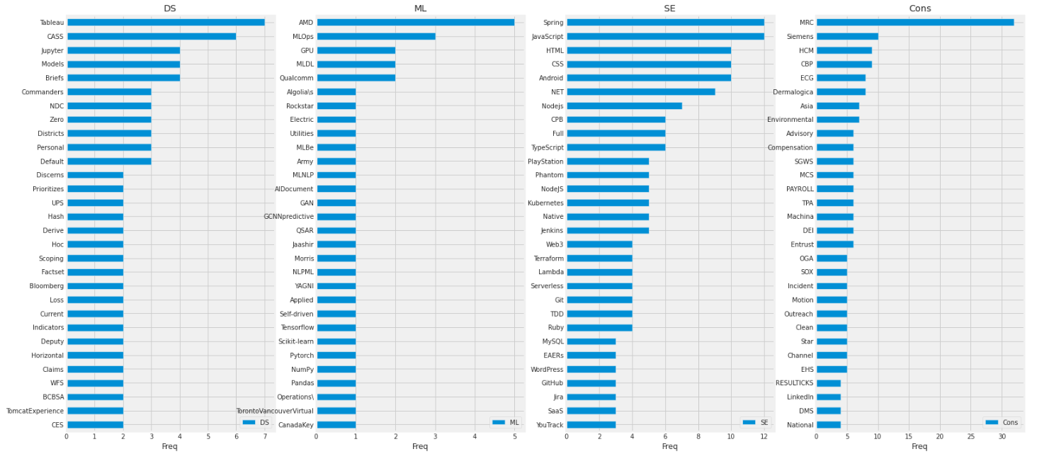
結果:
全体として結果を見ると、かなり職種をイメージ出来て納得感のある単語を抽出出来ているように感じた。(かなりラベルが小さくなってしまっているのでぜひとも拡大してみて頂きたいところです)
Tableauやjupyterは上位30件の中ではDSにしか出現しなかった。また、SEではspringやjavascript,Andoroidなど開発言語/フレームワークが特有の単語として見られ、その上件数も比較的多くみられた。Consでは、他3職種と比べ、MRC,HCMなどのような用語があり、技術用語は少なかった。
単語の出現に基づく職種の予測(ルールベース)
各職種に特有な単語の出現に基づいた予測を行い、submissionまで行う。
手順は以下の通り。
- Trainデータから、職種ごとに出現単語を抽出する
- 職種ごとの出現単語の内、n個以上の職種で出現しない単語を抽出する
- n=3としたとき、他の3職種以上で出現しない単語を抽出する
- Testデータに対して、上記で抽出した単語の出現数を計算し、最も出現数が多かった職種を予測値とする
なお、Train/Testデータ両方で職種特有の単語がテキスト中にないデータがあるため、それらのデータは職種特有の単語に限定せずに出現数を数えて補完している。
def rule_predict(df, words_by_job):
  """textごとにwords_by_jobの単語が出現するかを職種別に計算する
  """
  word_counts_all = []
  for text in df["description"]:
    word_counts_row = []
    for str_flag, words in words_by_job.items():
      word_count = sum(word in text for word in words)
      word_counts_row.append(word_count)
    word_counts_all.append(word_counts_row)
  pred = pd.DataFrame(word_counts_all, columns=list(words_by_job.keys()), index=df.index)
  return pred
target_pos = ["NN", "NNS", "NNP", "NNPS", "VB", "VBD", "VBG", "VBN", "VBP", "VBZ", "JJ", "JJR", "JJS", "RB", "RBR", "RBS"]
unique_words_by_job = calculate_unique_words_by_job(preprocess_train, re_labels, target_pos=target_pos, n=3)
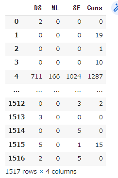
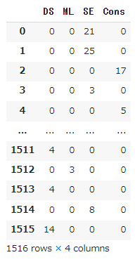
Testデータに対する予測
# testに対する予測
pred_test = rule_predict(preprocess_test, unique_words_by_job)
# 職種特有の単語が一つも出現しないデータを抽出
pre0_index = pred_test[(pred_test ==  0).all(axis=1)].index
# pre0_index
# どの職種で出現しても良い条件で単語を抽出
words_by_job_for_complement = calculate_unique_words_by_job(preprocess_train, re_labels, target_pos=target_pos, n=0)

# 職種特有の単語が出現しないデータを、補完用の予測に置き換え
complement_test = rule_predict(preprocess_test.iloc[pre0_index], words_by_job_for_complement)
pred_test.iloc[pre0_index] = complement_test
pred_test
sample = pd.read_csv("/content/drive/MyDrive/SIGNATE/studentcup2022summer/dataset/submit_sample.csv", header=None)
sample[1] = np.argmax(pred_test.values,axis=1) + 1
sample.to_csv(f'/content/drive/MyDrive/SIGNATE/studentcup2022summer/submission.csv', index=False, header=None)
# sample
結果は...
LB:0.5197424と数値的にはおよそ半分ほどでした;;
Trainデータに対する評価
結果は0.928728。
# trainに対する予測
pred_train = rule_predict(preprocess_train, unique_words_by_job)
# 職種特有の単語が一つも出現しないデータを抽出
pre0_index = pred_train[(pred_train ==  0).all(axis=1)].index
# pre0_index
# どの職種で出現しても良い条件で単語を抽出
words_by_job_for_complement = calculate_unique_words_by_job(preprocess_train, re_labels, target_pos=target_pos, n=0)

# 職種特有の単語が出現しないデータを、補完用の予測に置き換え
complement_train = rule_predict(preprocess_train.iloc[pre0_index], words_by_job_for_complement)
pred_train.iloc[pre0_index] = complement_train
pred_train
from sklearn.metrics import f1_score

le_labels = {"DS": 1, "ML": 2, "SE": 3, "Cons": 4}
f1_score(train["jobflag"].map(le_labels).values, np.argmax(pred_train.values, axis=1)+1, average='macro')
# 0.9287280420450924
結果について:
4択の問題で指標的には半分に到達してるので、ランダムの結果よりは良いと思います。今回、検証データによる評価は行っていませんが、Trainでの評価が0.92程度に対して、Test(LB)の値が0.51とかなり差がありますし、手法的にも、汎化にはかなり難はあると思います。
しかし、職種特有の固有名詞分析で判明した単語に納得する部分もあるかと思います。
例えば、求人の内、前半部分は似たような内容で、後半部分は必要となるスキルが少しだけ記載されている場合があるとします。MLによる予測でどの程度微妙な変化を吸収できるか不明ですが、もし後の微妙な違いが読み取れなかったとしたら、今回判明した職種別に特有な単語などに基づいて、後処理的に予測値を調整することも用途として考えられそうかなと思いました。
以上になります!!