Amsterdamに泊まりたい人のためにAirbnbのデータを分析したから

Amserdamに泊まりたいかーー

オランダの首都アムステルダムは街並みが非常に綺麗で、とても有名な観光地です。ヨーロッパでも特に特徴的な運河がたくさんある街であり、観光客が多すぎるのが問題になっちゃうくらい観光場所として有名です。

Airbnb

Airbnbといえば有名な民泊サービスです。Air bedとBed&BreakfastというところからAirbnbは来てます。ブライアン・チェスキーが自宅のロフトをお金のたまに貸し出したところから始まったといわれるサービスですね。海外では主流の宿泊先です。

目的

アムステルダム観光客がAirbnbに宿泊しようとする際にAirbnbの状況を把握してほしいという目的。
今回はアムステルダムのAirbnb宿泊先データを分析し、どのような特徴があるのか、どの変数がAirbnb宿泊の価格に影響しているのかなどを知るために分析をしました。

対象データ

[Inside Airbnb -Adding data to the debate]
http://insideairbnb.com/get-the-data.html
Inside AirbnbとはAirbnbの実際のデータを提供してくれているサイトである。
非常に整ったデータでcsv形式で提供してくれているので僕みたいな初心者でも分析しやすいよう担っている。

*今回はJupyter-Notebookで進めていきます。
*細かいデータ下処置など少し飛ばしています。

参考

https://towardsdatascience.com/exploring-machine-learning-for-airbnb-listings-in-toronto-efdbdeba2644
https://note.com/ryohei55/n/n56f723bc3f90

時系列データ分析

calendar = pd.read_csv('calendar.csv')
print(calendar.date.nunique(), 'days', calendar.listing_id.nunique(), 'unique listings')

366 days 20025 unique listings
2020-12-08から2020-12-06までのデータなのですがなぜか366daysといういきなり少し誤差がみられますが、データをみた限り問題なさそうなので進めます。20025listingsもありデータ量は多くありありがたいですね。

calendar.head(5)

予約できるかグラフ

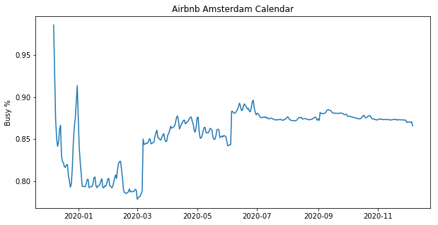
すでにどのくらいAirbnbが予約済みで、空きがあるのかを時系列にそってグラフ化してみました。

calendar_new = calendar[['date', 'available']]
calendar_new['busy'] = calendar_new.available.map( lambda x:0 if x == 't'  else 1)
calendar_new = calendar_new.groupby('date')['busy'].mean().reset_index()
calendar_new['date'] = pd.to_datetime(calendar_new['date'])

plt.figure(figsize=(10, 5))
plt.plot(calendar_new['date'], calendar_new['busy'])
plt.title('Airbnb Amsterdam Calendar')
plt.ylabel('Busy %')
plt.show()

考察
全体として80%以上の満室率なのでアムステルダムのairbnbは年中を通して混雑していると認識できる。
年越しにかけては非常に混雑をする。年越しの花火などをみにくる観光客の影響などによるものが考えられる。

3月以降にも混雑率は上昇する。6月にも同じように突発的な上昇が見られる。
しかしこれら上昇はairbnbのホストが現時点から少し遠くの予約はホストの予定も決まっていない以上決められないため部屋を空けていないものとも考えられる。

月ごとの価格比較

calendar['date'] = pd.to_datetime(calendar['date'])
calendar['price'] = calendar['price'].str.replace('$', '')
calendar['price'] = calendar['price'].str.replace(',', '')
calendar['price'] = calendar['price'].astype(float)
calendar['date'] = pd.to_datetime(calendar['date'])

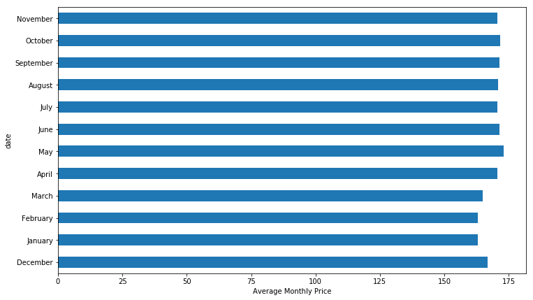
mean_of_month = calendar.groupby(calendar['date'].dt.strftime('%B'), sort=False)['price'].mean()

mean_of_month.plot(kind = 'barh', figsize=(12, 7))
plt.xlabel('Average Monthly Price')

考察
年中通してアムステルダムでのairbnbの平均価格は一泊160ユーロ(¥18000)くらいと言えます。強いていうなら1,2月が少し安そうという印象です。

曜日ごとの価格

calendar['dayofweek'] = calendar.date.dt.weekday_name
cats = [ 'Monday', 'Tuesday', 'Wednesday', 'Thursday', 'Friday', 'Saturday', 'Sunday']
price_week = calendar[['dayofweek', 'price']]
price_week = calendar.groupby(['dayofweek']).mean().reindex(cats)
price_week.drop(['listing_id','maximum_nights', 'minimum_nights'], axis=1, inplace=True)
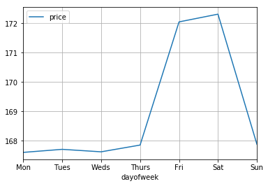
price_week.plot(grid=True)

ticks = list(range(0,7,1))
labels = "Mon Tues Weds Thurs Fri Sat Sun".split()
plt.xticks(ticks, labels)![download (14).png](https://qiita-image-store.s3.ap-northeast-1.amazonaws.com/0/505543/155809c6-0f06-2623-2d6e-78405d07ab30.png)

考察
月曜日から木曜日までは170ユーロ以下の平均で落ち着いているが、金曜日から土曜日にかけて宿泊する際は極端に値段が上がっている。学校や会社が休みの金曜土曜日曜にかけて旅行などで訪れるためairbnbの需要が週末に偏っているためと考えられる。

リスティングデータ分析

Airbnbそれぞれの宿泊先に関するデータが含まれている。

listings = pd.read_csv('listings.csv')
print('We have', listings.id.nunique(), 'listings in the listing data.')
listings.head(5)

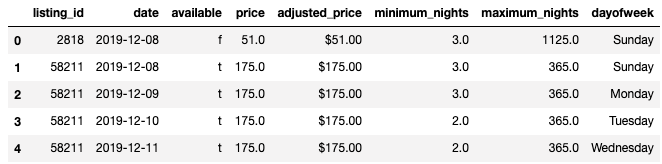
このような形になっている。

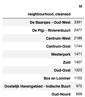
どこに宿泊先はあるかTOP10

listings.groupby(by = 'neighbourhood_cleansed').count()[['id']].sort_values(by='id', ascending=False).head(10)

価格分布

listings.loc[(listings.price <= 1000) & (listings.price > 0)].price.hist(bins=200)
plt.ylabel('Count')
plt.xlabel('Listing price in　EUR')
plt.title('Histogram of listing prices')

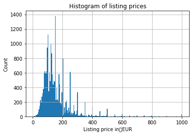
価格の分布はこのようになっています。

地域ごとの価格箱ひげ図

select_neighbourhood_over_100 = listings.loc[(listings.price <= 1000) & (listings.price > 0)].groupby('neighbourhood_cleansed')\
.filter(lambda x: len(x)>=100)["neighbourhood_cleansed"].values

listings_neighbourhood_over_100 = listings.loc[listings['neighbourhood_cleansed'].map(lambda x: x in select_neighbourhood_over_100)]

sort_price = listings_neighbourhood_over_100.loc[(listings_neighbourhood_over_100.price <= 1000) & (listings_neighbourhood_over_100.price > 0)]\
.groupby('neighbourhood_cleansed')['price'].median().sort_values(ascending=False).index

sns.boxplot(y='price', x='neighbourhood_cleansed', data=listings_neighbourhood_over_100.loc[(listings_neighbourhood_over_100.price <= 1000) & (listings_neighbourhood_over_100.price > 0)],
            order=sort_price)

ax = plt.gca()
ax.set_xticklabels(ax.get_xticklabels(), rotation=45, ha='right')
plt.show()

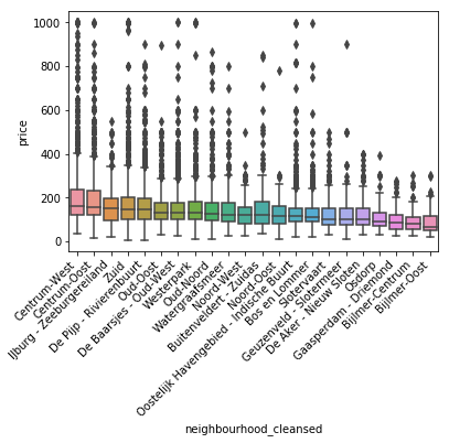
考察
Centrum-West Centrum-Oostにわかるように中央駅に近いところは流石に高い価格設定になっている。
Bijnmerのようにトラムで30分くらいかかる地区にいくと最も安い価格帯と言える。基本的に中央駅からの距離でその周辺のairbnbの価格は決まっていると言っても良さそうである。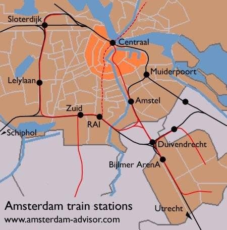

宿泊形態ごとの価格箱ひげ図

select_property_over_100 = listings.loc[(listings.price <= 1000) & (listings.price > 0)].groupby('property_type')\
.filter(lambda x:len(x) >=20)["property_type"].values

listings_property_over_100 = listings.loc[listings["property_type"].map(lambda x: x in select_property_over_100)]

sort_price = listings_property_over_100.loc[(listings_property_over_100.price <= 1000) & (listings_property_over_100.price >0)]\
.groupby('property_type')['price'].median().sort_values(ascending=False).index

sns.boxplot(y='price', x ='property_type', data=listings_property_over_100.loc[(listings_property_over_100.price <= 1000) & (listings_property_over_100.price >0)],
           order = sort_price)

ax = plt.gca()
ax.set_xticklabels(ax.get_xticklabels(), rotation=45, ha='right')
plt.show()

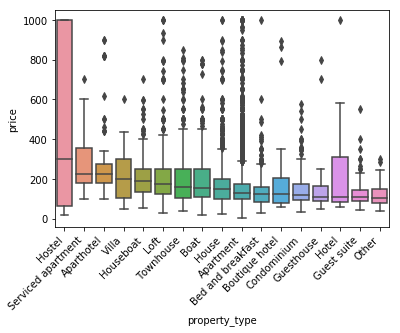
考察
まず箱ひげ図とはデータのばらつきを見るもので、中央の線が中央値を指しており、そこから下の濃い線が第一四分位数、その上の濃い線が第三四分位数となっています。
ホステルというのはヨーロッパではよくある格安に泊まることのできる宿舎です。しかし格安とはいえどホステルに分類はされてはいるもののアムステルダムでは1000EURに及ぶものも多くあるようです。しかし今回では1000EUR以上は外れ値として外してしまっているのも考慮しなければなりません。

Hotelもデータにばらつきがみられます。おそらく高級なテイストのホテルもあるためでしょう。しかし中央値自体は180EURくらいの場所にあるためHotelに分類されているairbnbは基本的には安い分類のようです。

部屋のタイプによる価格グラフ

listings.loc[(listings.price <= 1000) & (listings.price > 0)].pivot(columns='room_type', values='price').plot.hist(stacked=True, bins=100)
plt.xlabel('Listing Price in EUR')

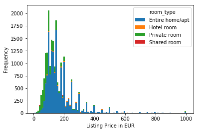
考察
まずShared roomとHotel roomがほとんどないことに気づきます。家・アパートごと貸し出しか、部屋だけ貸し出しのタイプです。そして多いのは家・アパートごと貸し出しのようです。
安く済ませたいならprivate roomに絞って探す方が効率は良さそうです。家・アパートごと貸し出しの場合は、当然ですが部屋だけ貸し出しより高くついてしまう結果になりそうです。

アメニティの数グラフ

pd.Series(np.concatenate(listings['amenities'].map(lambda amns: amns.split(",")))).value_counts().head(20).plot(kind='bar')
ax = plt.gca()
ax.set_xticklabels(ax.get_xticklabels(), rotation=45, ha='right', fontsize=12)
plt.show()

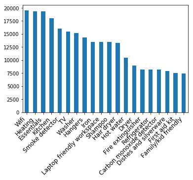
考察
Wifiは多いね。オランダの冬は寒いしHeatingももちろん装備しているところがほとんどです。
アイロンシャンプードライヤーなどのアメニティはないところも多いので少し確認が必要となってくるでしょう。

Family and kid friendlyは少なめですね...でもairbnbでは干渉されたくないというのが多いのでこれは利点とも考えられ明日ね。
またfree parkingが上位に入っていないことも見れるので、車で来る際はお気をつけください

価格とアメニティの関係性

amenities = np.unique(np.concatenate(listings['amenities'].map(lambda amns: amns.split(","))))
amenity_prices = [(amn, listings[listings['amenities'].map(lambda amns: amn in amns)]['price'].mean()) for amn in amenities if amn != ""]
amenity_srs = pd.Series(data=[a[1] for a in amenity_prices], index=[a[0] for a in amenity_prices])

amenity_srs.sort_values(ascending=False)[:20].plot(kind='bar')
ax = plt.gca()
ax.set_xticklabels(ax.get_xticklabels(), rotation=45, ha='right', fontsize=12)
plt.show()

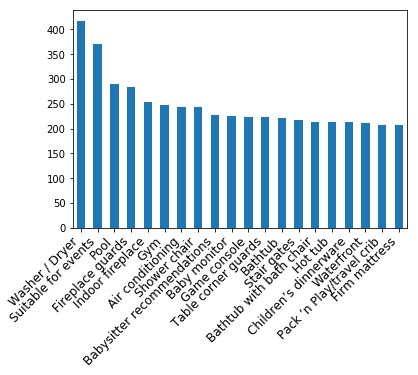
考察
Washer/Dryerがもっとも価格に関係しているというのは関連性はわからないです...
しかしアムステルダムらしいというのはSuitable for eventsですね。アムステルダムでは多くのイベントが開催されています。そのイベントに対して参加しやすかったり、適切な場所にあったりする部屋が高くなる傾向にあるようです。その2つ以外は一律に近い関連性ですね。

ベッドの数と価格の関連性

listings.loc[(listings.price <= 1000)&(listings.price > 0)].pivot(columns = 'beds', values='price').plot.hist(stacked=True, bins=100)
plt.xlabel('Listing price in EUR')

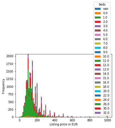
考察
ほとんどベッドが1個か2個ですね。これに関してはイメージ通りの結果ですかね。
ちなみにベッド32個！？って思ったのでみてみると。
https://www.airbnb.jp/rooms/779175?source_impression_id=p3_1577402659_vntGlW7Yj5I5pX4U
このフェリーをのベッドが32個あると言う話でした。びっくりですね。

ヒートマップでアメニティ同士の関連性を視覚化

col = ['host_listings_count', 'accommodates', 'bedrooms', 'price', 'number_of_reviews', 'review_scores_rating']
corr = listings.loc[(listings.price<=1000)&(listings.price > 0)][col].dropna().corr()
plt.figure(figsize=(6,6))
sns.set(font_scale=1)
sns.heatmap(corr, cbar=True, annot=True, square=True, fmt='.2f', xticklabels=col, yticklabels=col)
plt.show()

考察
これはlistingsデータ内それぞれの相関を色でみやすいようにしたものでヒートマップと言われています。しかし今回に限っては、ほとんどの部分で相関はみられないですね。
しかしbedroomsとaccommodatesには強めの相関が見られます。これは泊まれる人数とベッドの数なので相関があるのは納得ができます。しかしこのようにベッドの数によってaccomodatesの数を決めているようなものは相関関係があると言うよりは、人為的に宿泊人数をベッドの数として決めているので疑似相関と考えられます。

決定木を使って価格を予測

以下はデータ下処理です。データをダミー変数化したりしています。

from sklearn.feature_extraction.text import CountVectorizer

count_vectorizer = CountVectorizer(tokenizer=lambda x:x.split(','))
amenities = count_vectorizer.fit_transform(listings['amenities'])
df_amenities = pd.DataFrame(amenities.toarray(), columns=count_vectorizer.get_feature_names())
df_amenities = df_amenities.drop('', 1)

columns = ['host_is_superhost', 'host_identity_verified', 'host_has_profile_pic', 'is_location_exact', 'requires_license', 'instant_bookable', 'require_guest_profile_picture', 'require_guest_phone_verification']
for c in columns:
    listings[c] = listings[c].replace('f',0,regex=True)
    listings[c] = listings[c].replace('t',1,regex=True)

listings['security_deposit'] = listings['security_deposit'].fillna(value=0)
listings['security_deposit'] = listings['security_deposit'].replace('[\$,]', '', regex=True).astype(float)
listings['cleaning_fee'] = listings['cleaning_fee'].fillna(value=0)
listings['cleaning_fee'] = listings['cleaning_fee'].replace('[\$,]', '', regex=True).astype(float)

listings_new = listings[['host_is_superhost', 'host_identity_verified', 'host_has_profile_pic','is_location_exact', 
                         'requires_license', 'instant_bookable', 'require_guest_profile_picture', 
                         'require_guest_phone_verification', 'security_deposit', 'cleaning_fee', 
                         'host_listings_count', 'host_total_listings_count', 'minimum_nights',
                     'bathrooms', 'bedrooms', 'guests_included', 'number_of_reviews','review_scores_rating', 'price']]

for col in listings_new.columns[listings_new.isnull().any()]:
    listings_new[col] = listings_new[col].fillna(listings_new[col].median())

for cat_feature in ['zipcode', 'property_type', 'room_type', 'cancellation_policy', 'neighbourhood_cleansed', 'bed_type']:
    listings_new = pd.concat([listings_new, pd.get_dummies(listings[cat_feature])], axis=1)

listings_new = pd.concat([listings_new, df_amenities], axis=1, join='inner')

RandomForestRegressorを使っていきます。

from sklearn.model_selection import train_test_split
from sklearn.metrics import r2_score
from sklearn.metrics import mean_squared_error
from sklearn.ensemble import RandomForestRegressor

y = listings_new['price']
x = listings_new.drop('price', axis=1)
X_train, X_test, y_train, y_test = train_test_split(x, y, test_size=0.25, random_state=123)
rf = RandomForestRegressor(n_estimators=500, random_state=123, n_jobs=-1)
rf.fit(X_train, y_train)
y_train_pred = rf.predict(X_train)
y_test_pred = rf.predict(X_test)
rmse_rf = (mean_squared_error(y_test, y_test_pred))**(1/2)

print('RMSE test: %.3f' % rmse_rf)
print('R^2 test: %.3f' % (r2_score(y_test, y_test_pred)))

RMSE test: 73.245
R^2 test: 0.479
結果はこのようになりました。R^2テストで0.479ということでまぁまぁの精度ですね。とりあえず、決定木がどの項目を重要だと判断したのかについてみていきます。

coefs_df = pd.DataFrame()
coefs_df['est_int'] = X_train.columns
coefs_df['coefs'] = rf.feature_importances_
coefs_df.sort_values('coefs', ascending=False).head(20)

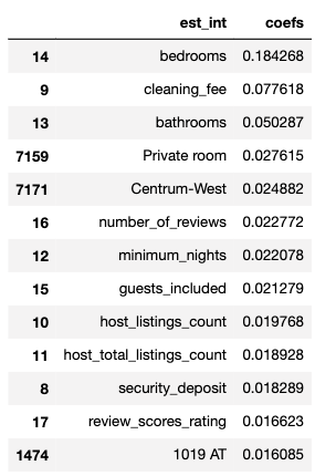
考察
ベッドルームがいくつあるかがかなり価格に影響しているのがわかる。またairbnbでは部屋代と別にクリーニング代が請求されるが、その代金も価格に影響しているのがわかる。これはかなり直接的に影響していると考えれる。

Lasso回帰

from sklearn.linear_model import  Lasso
lasso = Lasso()
lasso.fit(X_train, y_train)

# 回帰係数
print(lasso.coef_)
# 切片 (誤差)
print(lasso.intercept_)
# 決定係数
print(lasso.score(X_test, y_test))

[ 1.85022916e-03 1.31073590e+00 -0.00000000e+00 0.00000000e+00
5.23464952e+00 5.97640655e-01 6.42296851e-01 3.67942959e+01
8.80302532e+00 -3.96520183e-02 8.39294507e-01]
-30.055848397234712
0.27054071146797

重回帰分析なども試みてみましたが、あまり精度を高くすることはできませんでした。まあそりゃダミー変数化などしてるからこれは仕方ないよね？だよね？？

まとめ

データ分析を学びたてですが、このInside Airbnbというところでは非常に整ったデータが並べられており、初心者としてはありがたかったです。このように分析したいな！というオープンデータを探すのは少し難しいのでぜひ参考にしてみてください。

今回はかなり写しただけな部分も多いですが、それでも何を意図してどのようにデータ処理をするのかが学べたのでよかったです。

アドバイスなどいただけたらありがたいです！